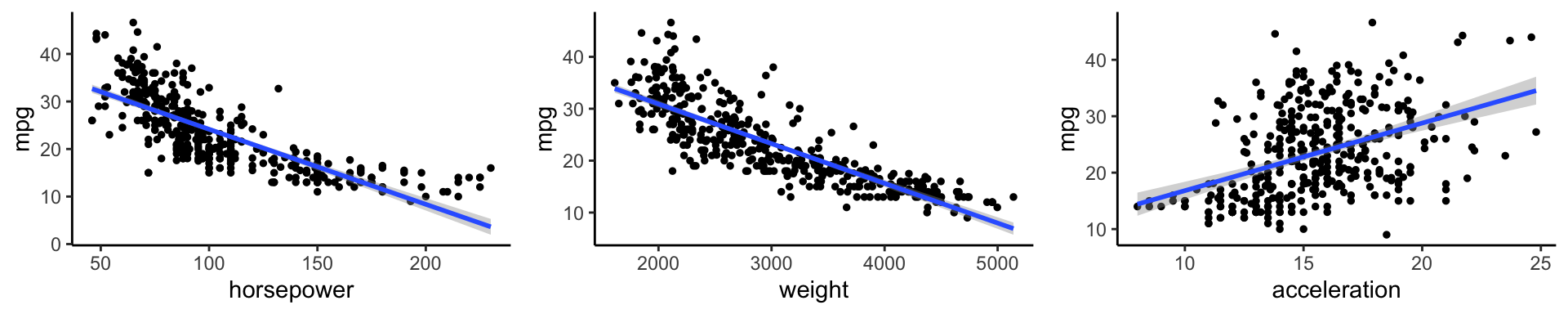
Above are mpg vs horsepower, weight, and acceleration, with a blue linear-regression line fit separately to each. Can we predict mpg using these three?
Assume for a moment that both \(\hat{f}\) and X are fixed.
\(E(Y − \hat{Y})^2\) represents the average, or expected value, of the squared difference between the predicted and actual value of Y, and Var( \(\varepsilon\) ) represents the variance associated with the error term
The focus of this class is on techniques for estimating f with the aim of minimizing the reducible error.
the irreducible error will always provide an upper bound on the accuracy of our prediction for Y
This bound is almost always unknown in practice
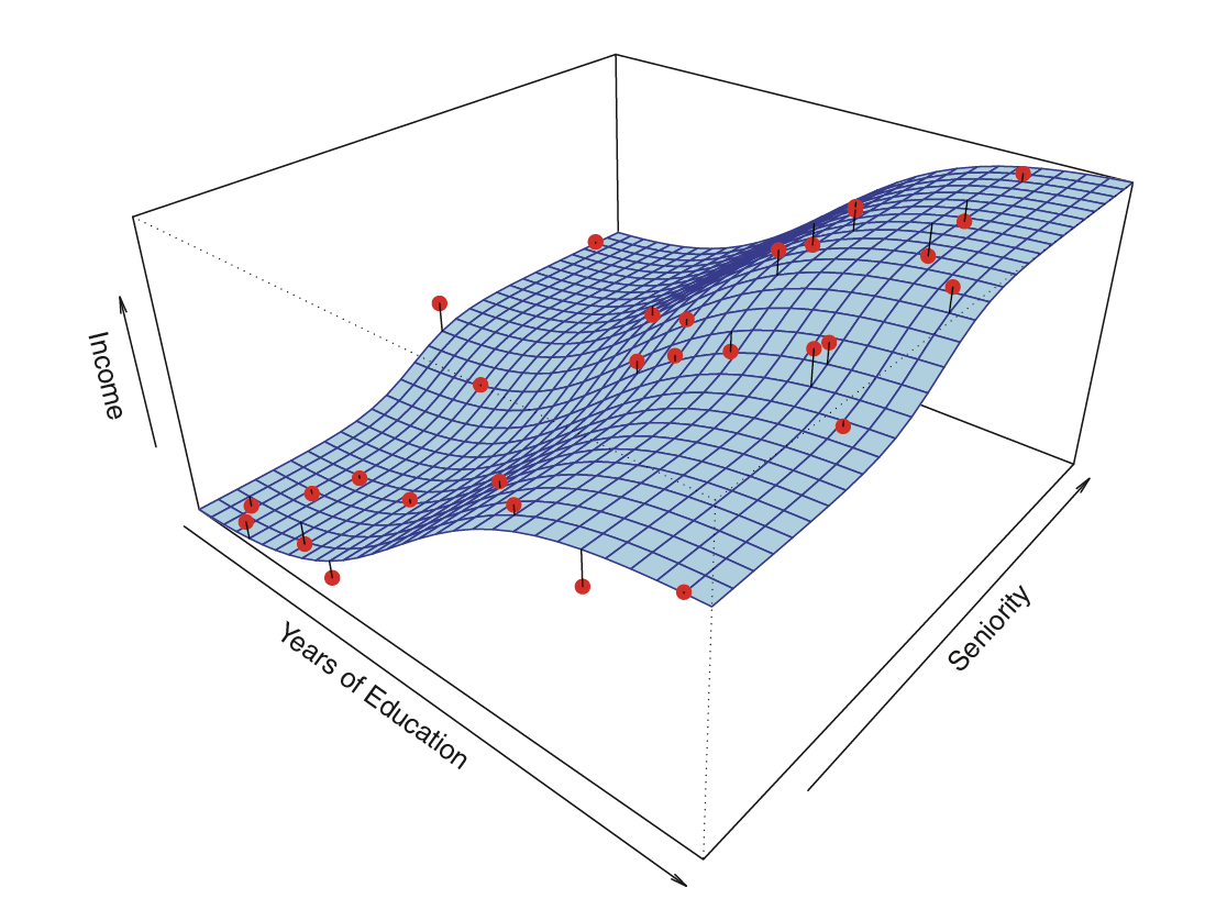
Estimating \(f\)
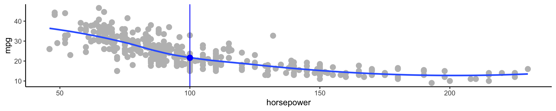
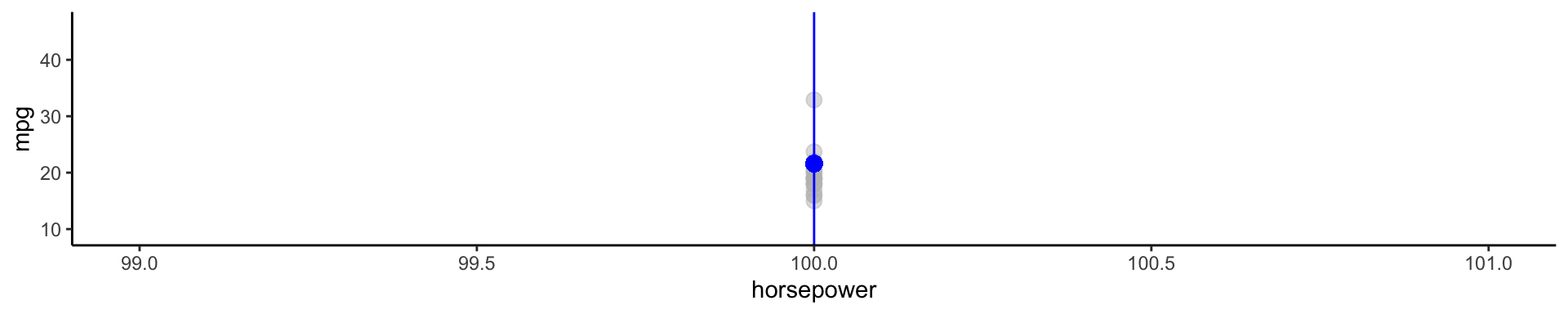
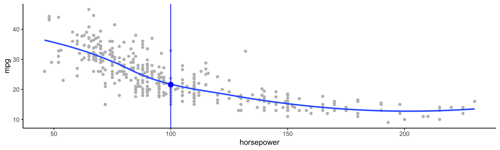
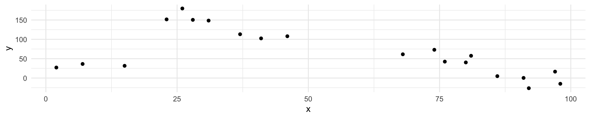
Typically we have very few (if any!) data points at \(X=x\) exactly, so we cannot compute \(E[Y|X=x]\)
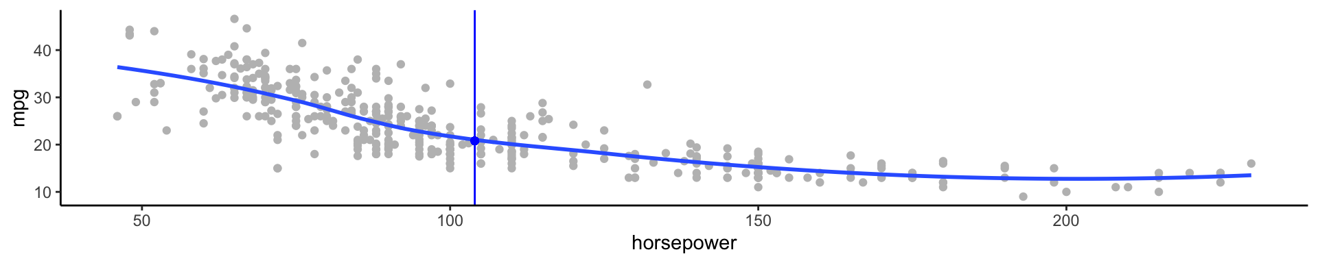
For example, what if we were interested in estimating miles per gallon when horsepower was 104.
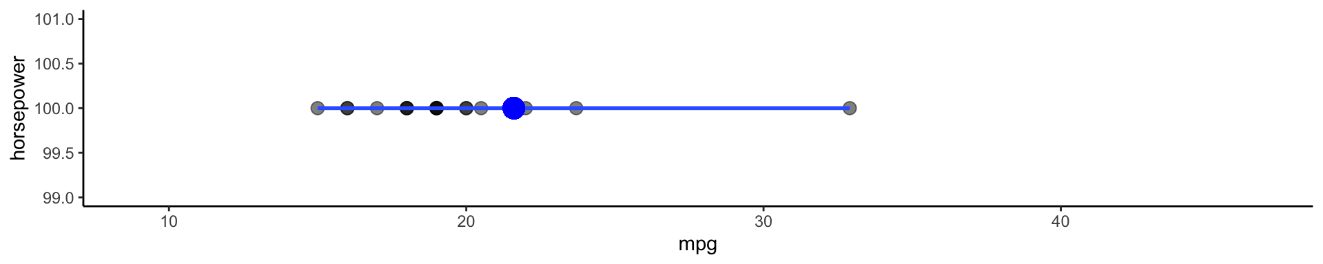
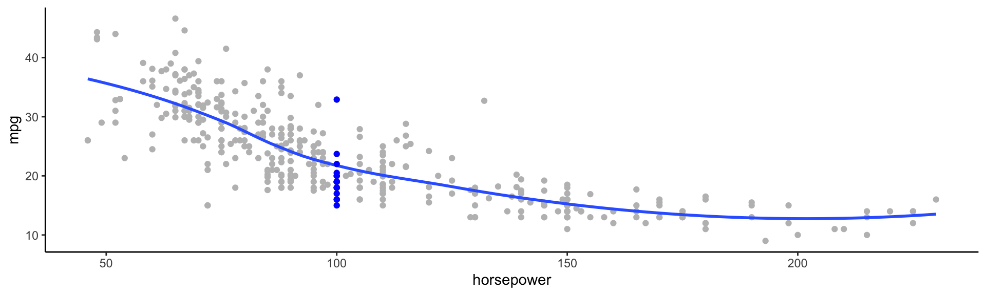
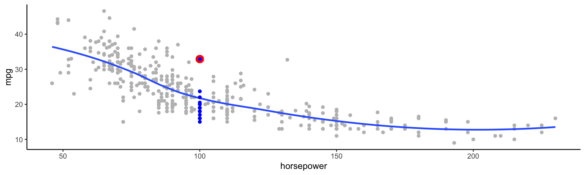
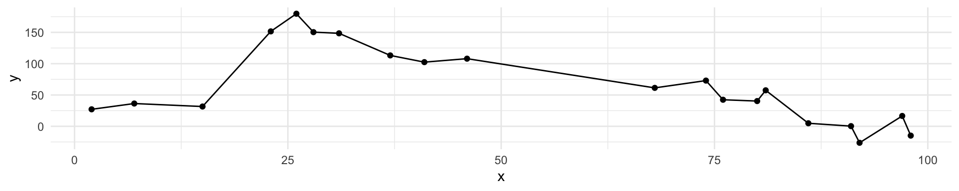
💡 We can relax the definition and let
\[\hat{f}(x) = E[Y | X\in \mathcal{N}(x)]\]
Where \(\mathcal{N}(x)\) is some neighborhood of \(x\)
Notation pause!
\[\hat{f}(x) = \underbrace{E}_{\textrm{The expectation}}[\underbrace{Y}_{\textrm{of Y}} \underbrace{|}_{\textrm{given}} \underbrace{X\in \mathcal{N}(x)}_{\textrm{X is in the neighborhood of x}}]\]
🚨 If you need a notation pause at any point during this class, please let me know!
Estimating \(f\)
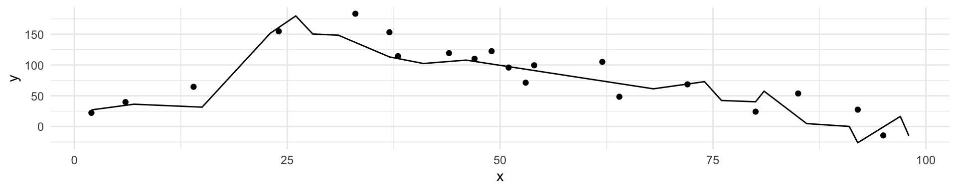
💡 We can relax the definition and let
\[\hat{f}(x) = E[Y | X\in \mathcal{N}(x)]\]
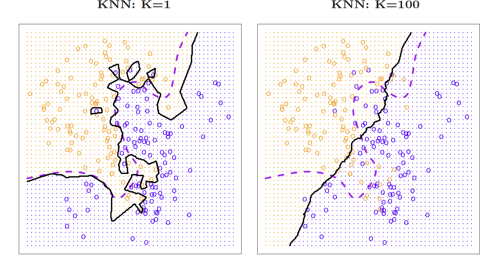
Nearest neighbor averaging does pretty well with small \(p\) ( \(p\leq 4\) ) and large \(n\)
Nearest neighbor is not great when \(p\) is large because of the curse of dimensionality (because nearest neighbors tend to be far away in high dimensions)
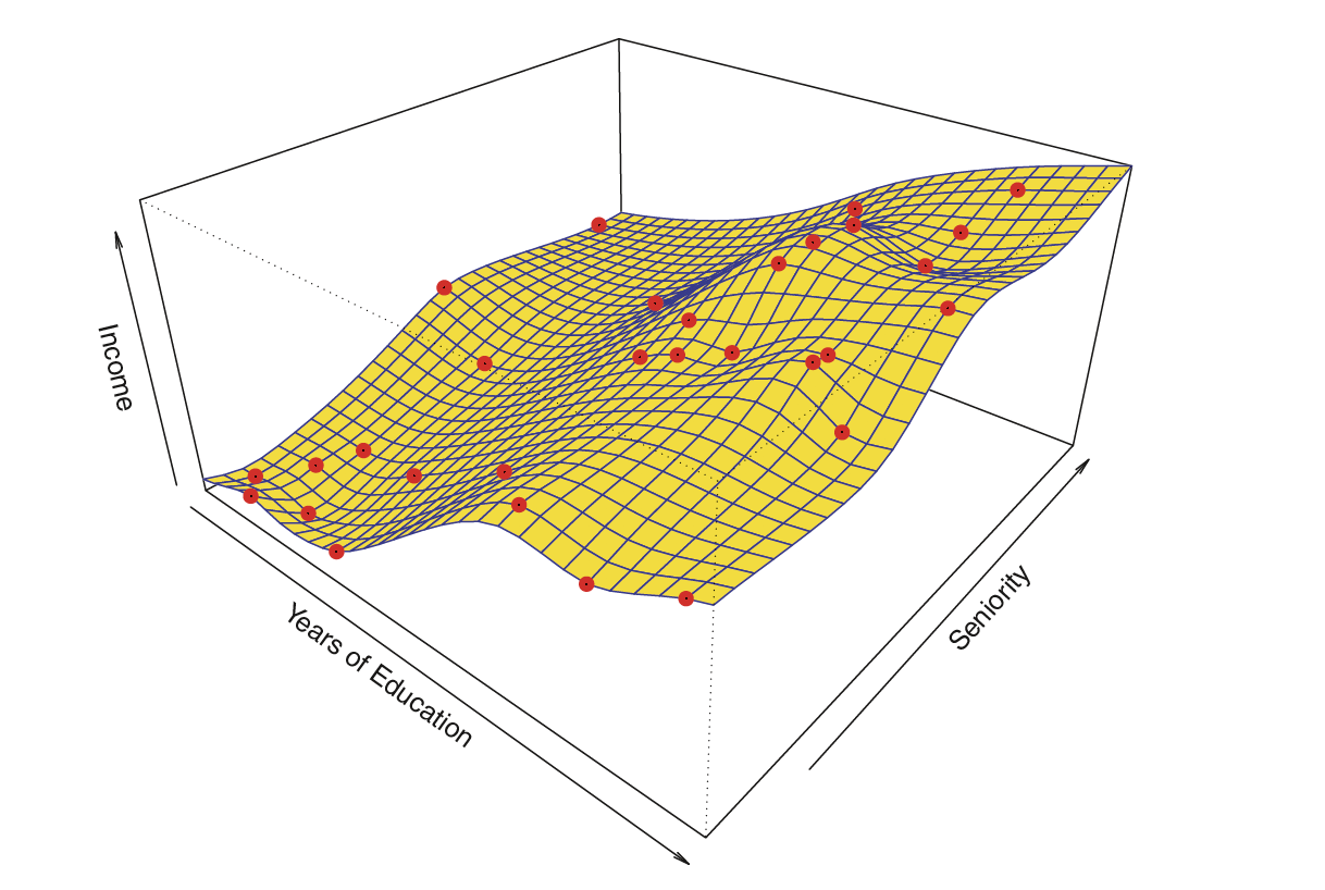
If we get a new sample, that overfit model is probably going to be terrible!
Accuracy
We’ve fit a model \(\hat{f}(x)\) to some training data \(\texttt{train} = \{x_i, y_i\}^N_1\)
Instead of measuring accuracy as the average squared prediction error over that train data, we can compute it using fresh test data \(\texttt{test} = \{x_i,y_i\}^M_1\)
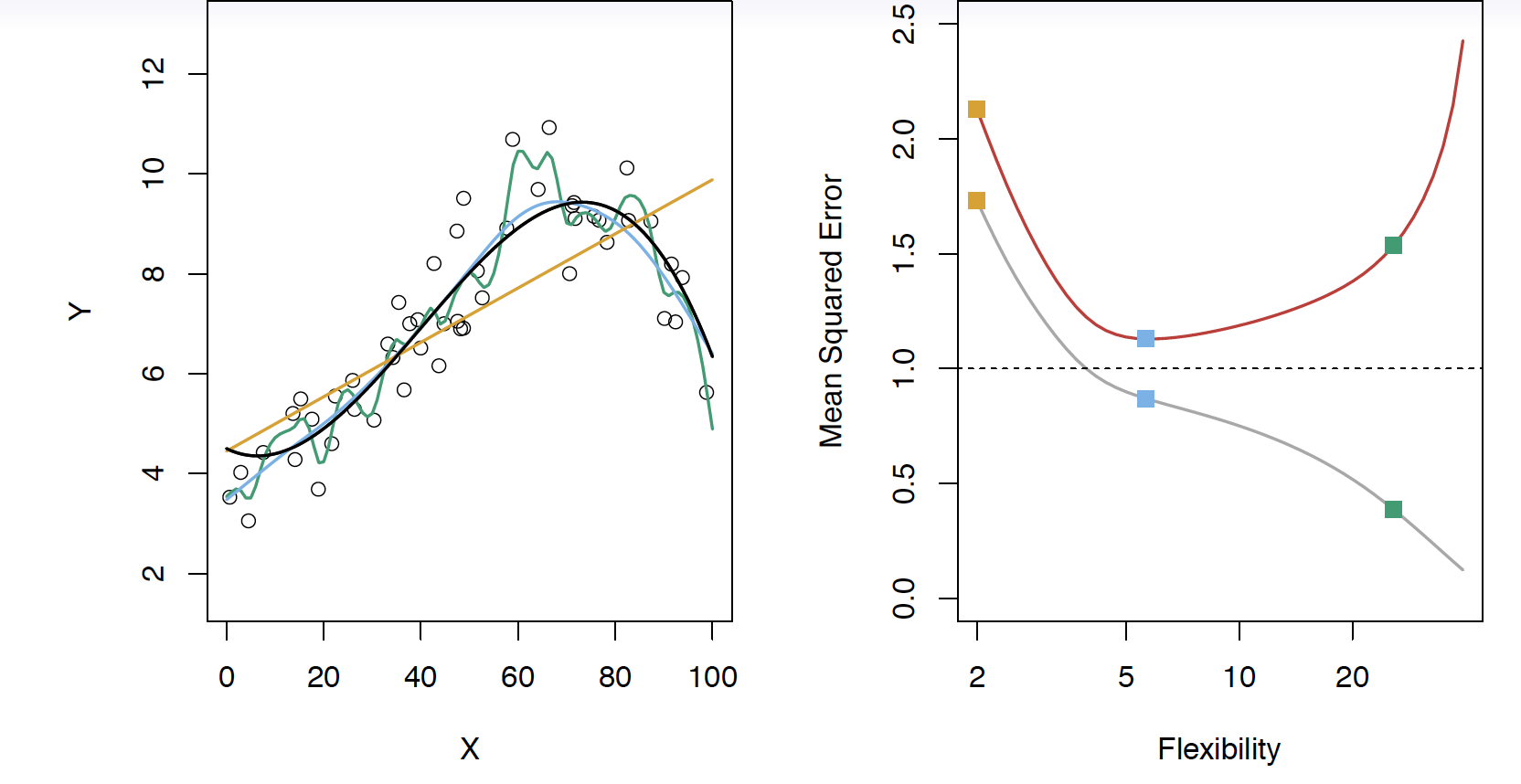
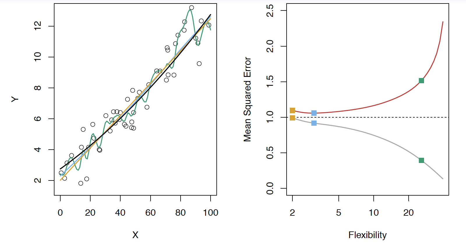
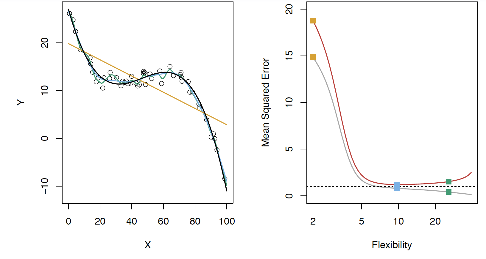
Black curve is the “truth” on the left. Red curve on right is \(MSE_{\texttt{test}}\), grey curve is \(MSE_{\texttt{train}}\). Orange, blue and green curves/squares correspond to fis of different flexibility.
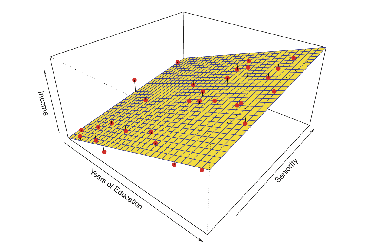
Here the truth is smoother, so the smoother fit and linear model do really well
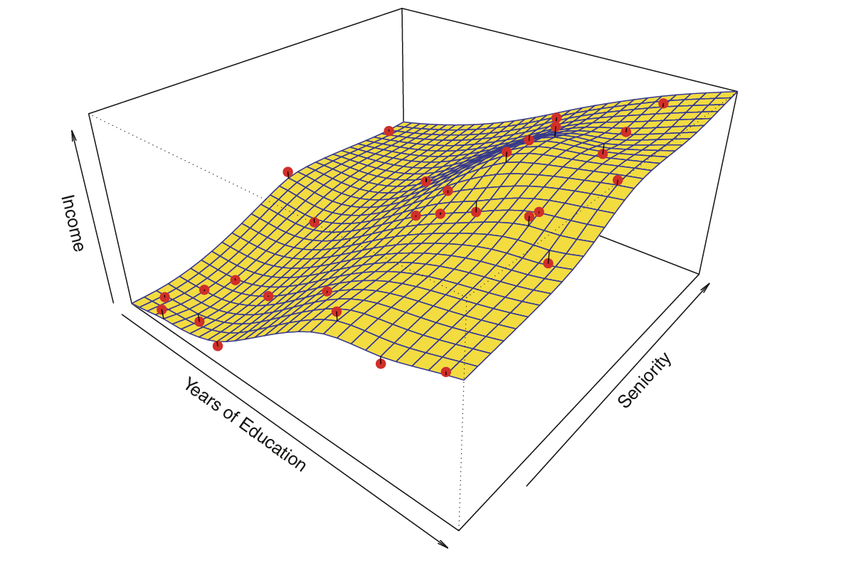
Here the truth is wiggly and the noise is low, so the more flexible fits do the best
Bias-variance trade-off
We’ve fit a model, \(\hat{f}(x)\), to some training data
Let’s pull a test observation from this population ( \(x_0, y_0\) )
The expectation averages over the variability of \(y_0\) as well as the variability of the training data. \(\textrm{Bias}(\hat{f}(x_0)) =E[\hat{f}(x_0)]-f(x_0)\)
As flexibility of \(\hat{f}\)\(\uparrow\), its variance \(\uparrow\) and its bias \(\downarrow\)
choosing the flexibility based on average test error amounts to a bias-variance trade-off
Bias-variance trade-off
Classification
Notation
\(Y\) is the response variable. It is qualitative
\(\mathcal{C}(X)\) is the classifier that assigns a class \(\mathcal{C}\) to some future unlabeled observation, \(X\)
Examples:
Email can be classified as \(\mathcal{C}=(\texttt{spam, not spam})\)
Written number is one of \(\mathcal{C}=\{0, 1, 2, \dots, 9\}\)
Classification Problem
What is the goal?
Build a classifier \(\mathcal{C}(X)\) that assigns a class label from \(\mathcal{C}\) to a future unlabeled observation \(X\)
Assess the uncertainty in each classification
Understand the roles of the different predictors among \(X = (X_1, X_2, \dots, X_p)\)
Suppose there are \(K\) elements in \(\mathcal{C}\), numbered \(1, 2, \dots, K\)
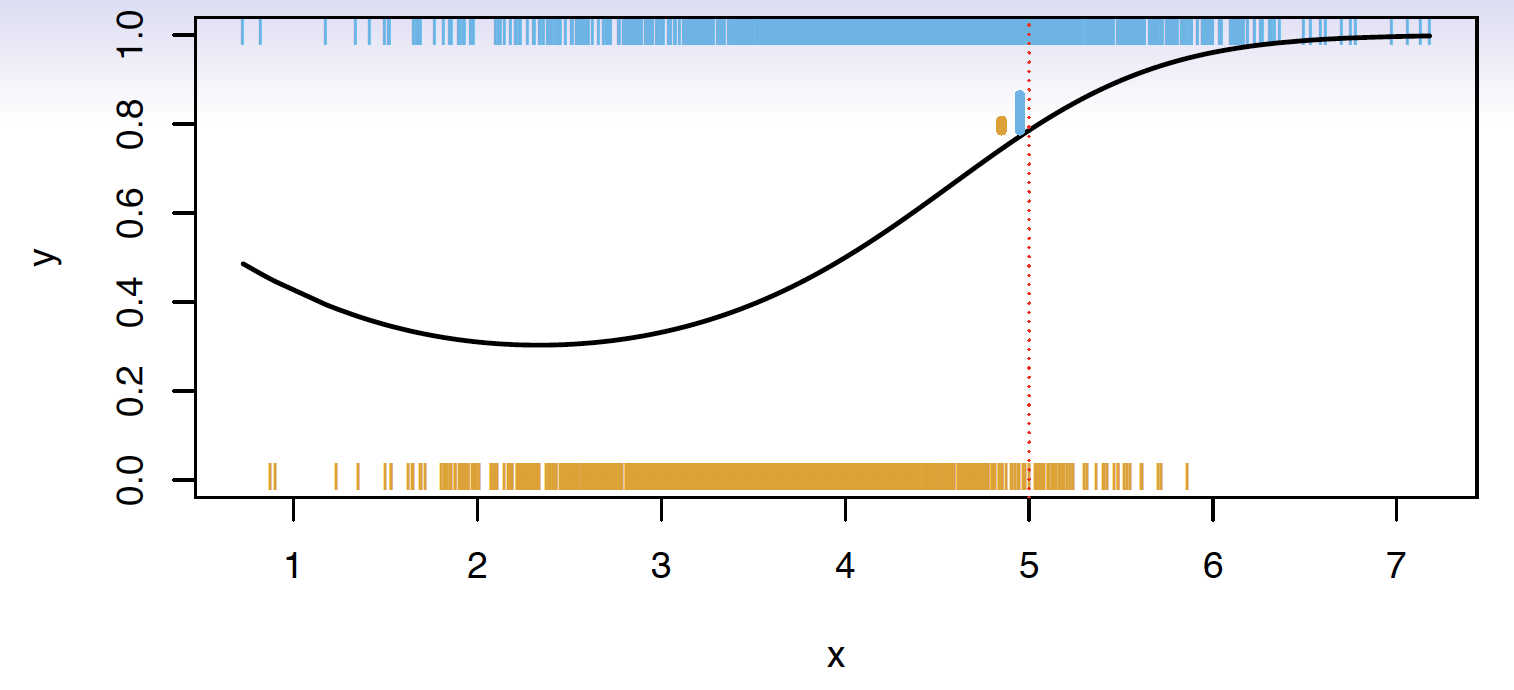
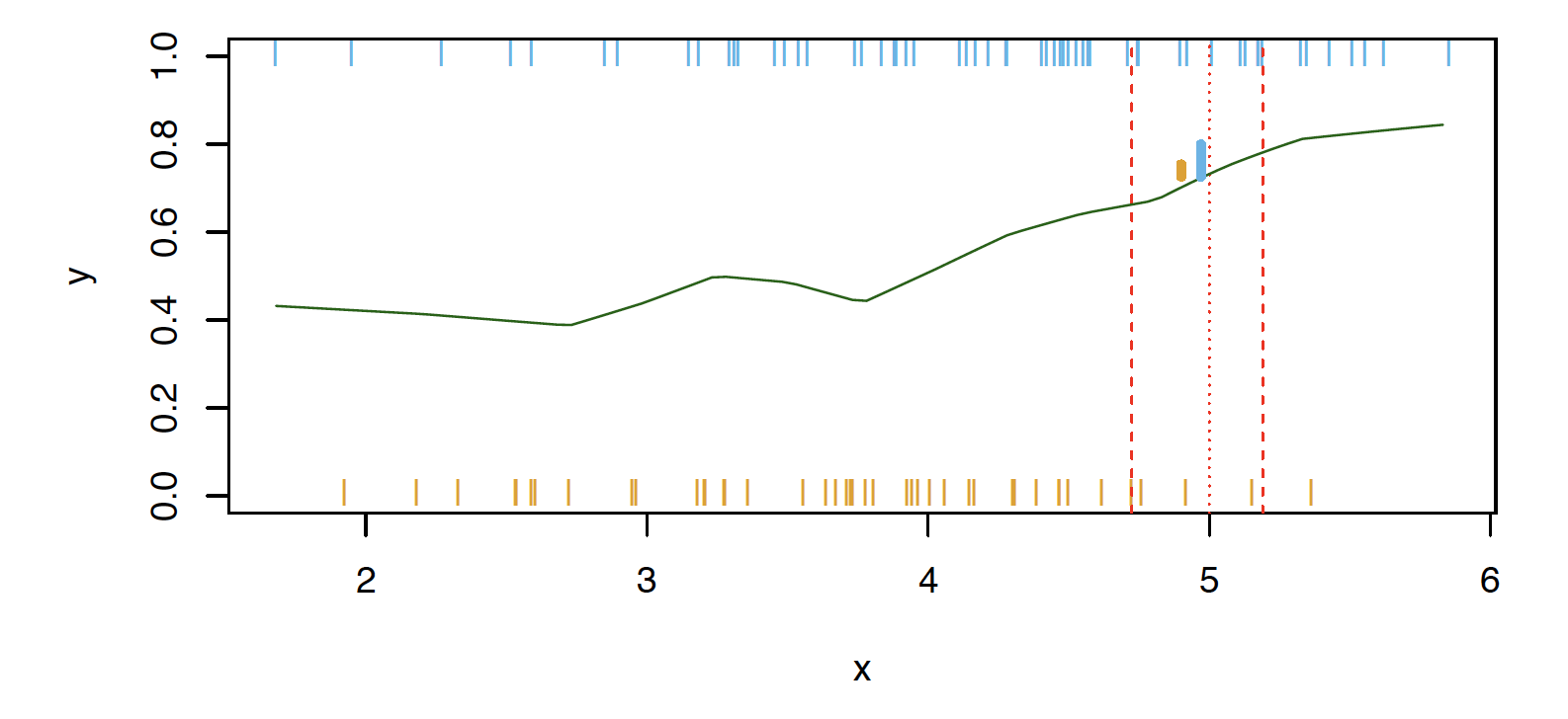
\[p_k(x) = P(Y = k|X=x), k = 1, 2, \dots, K\] These are conditional class probabilities at \(x\)
How do you think we could calculate this?
In the plot, you could examine the mini-barplot at \(x = 5\)
Suppose there are \(K\) elements in \(\mathcal{C}\), numbered \(1, 2, \dots, K\)
\[p_k(x) = P(Y = k|X=x), k = 1, 2, \dots, K\] These are conditional class probabilities at \(x\)