Exploratory Data Analysis
Reading in data
Some data is already loaded when you load certain packages in R, to access these, you just need to use the data() function like this:
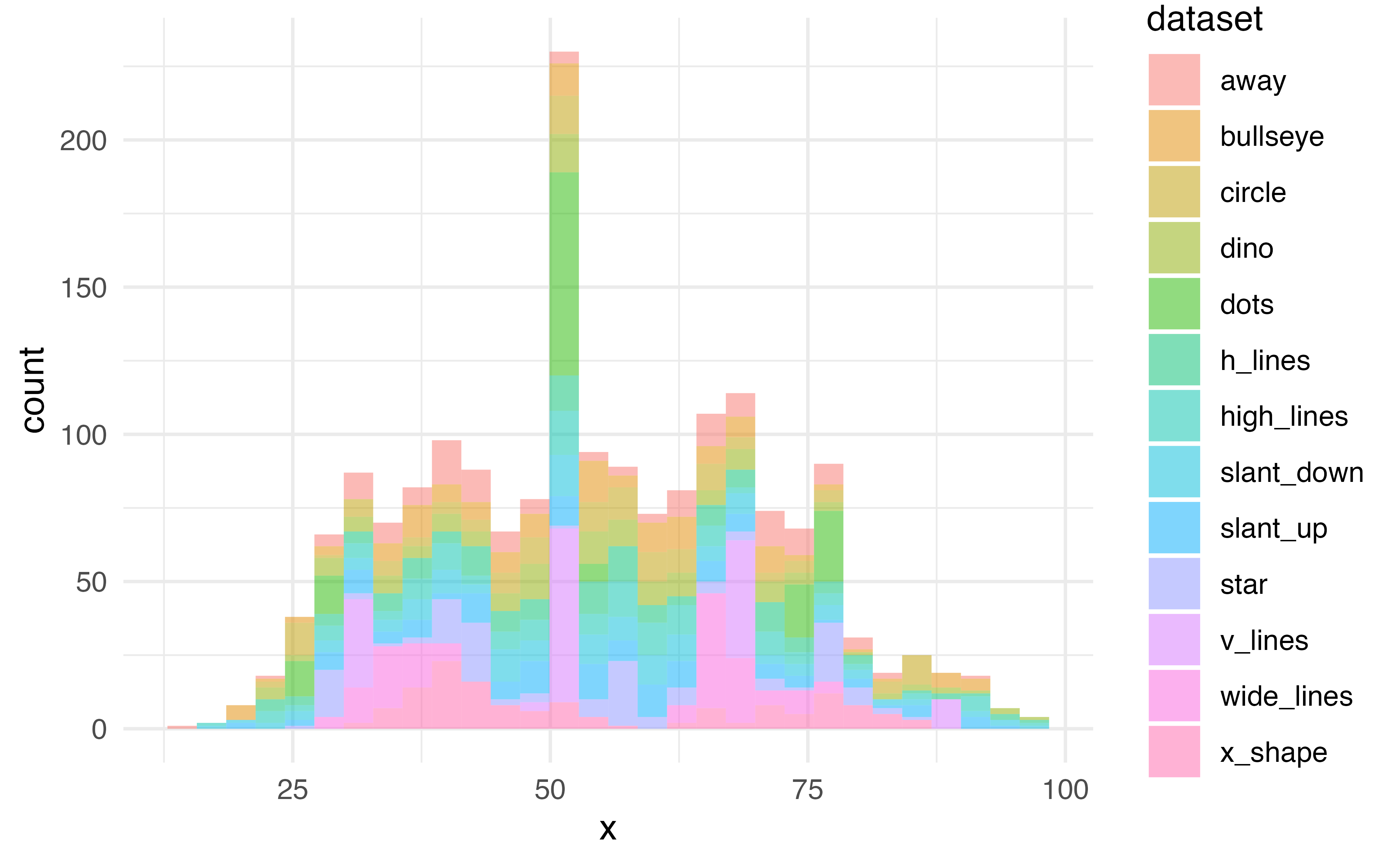
Histogram
What does this warning mean? How do you think we can get rid of it?
Histogram

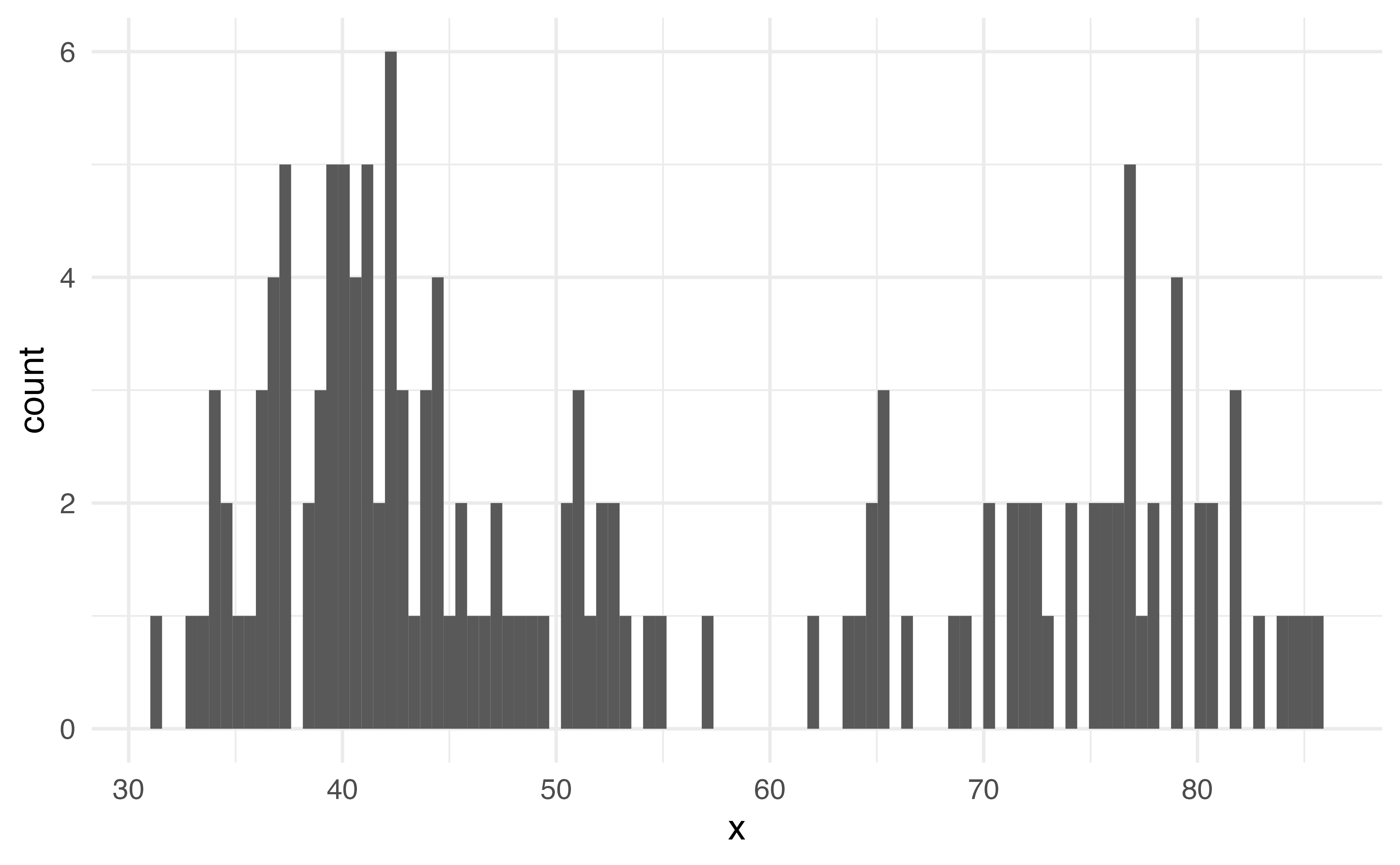

Histogram

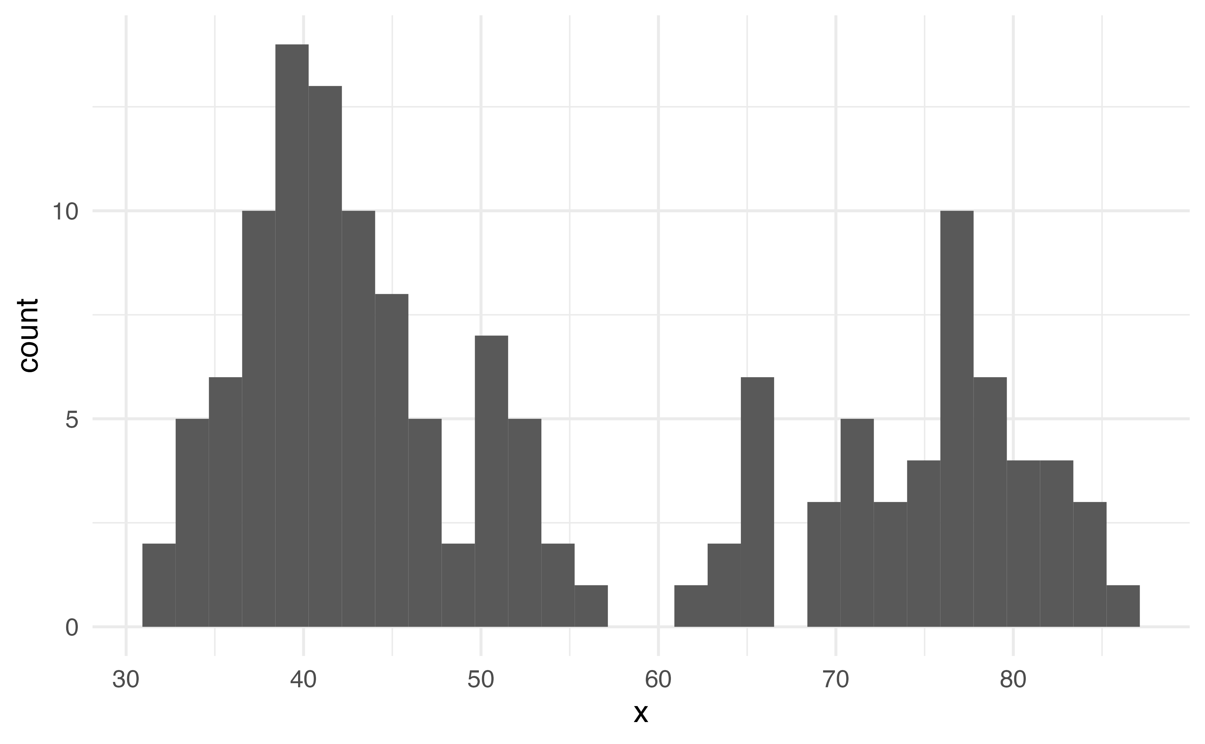
What does this plot tell us about the shape of this data?
00:30
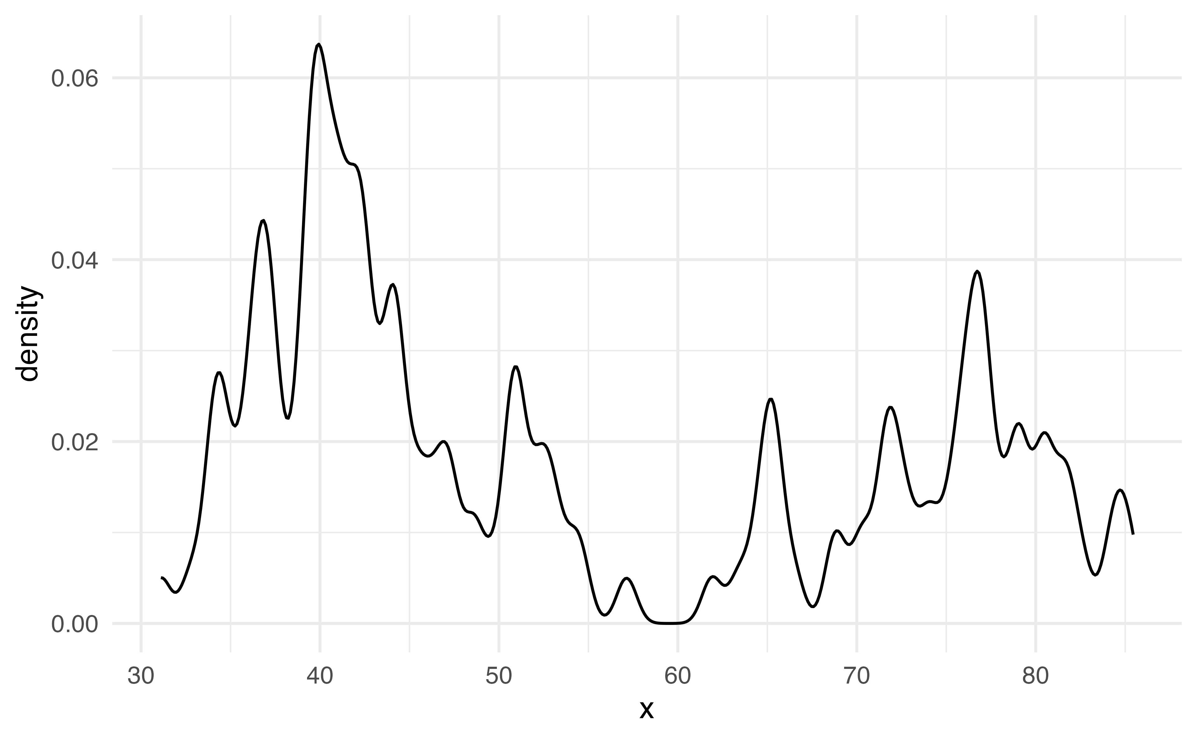
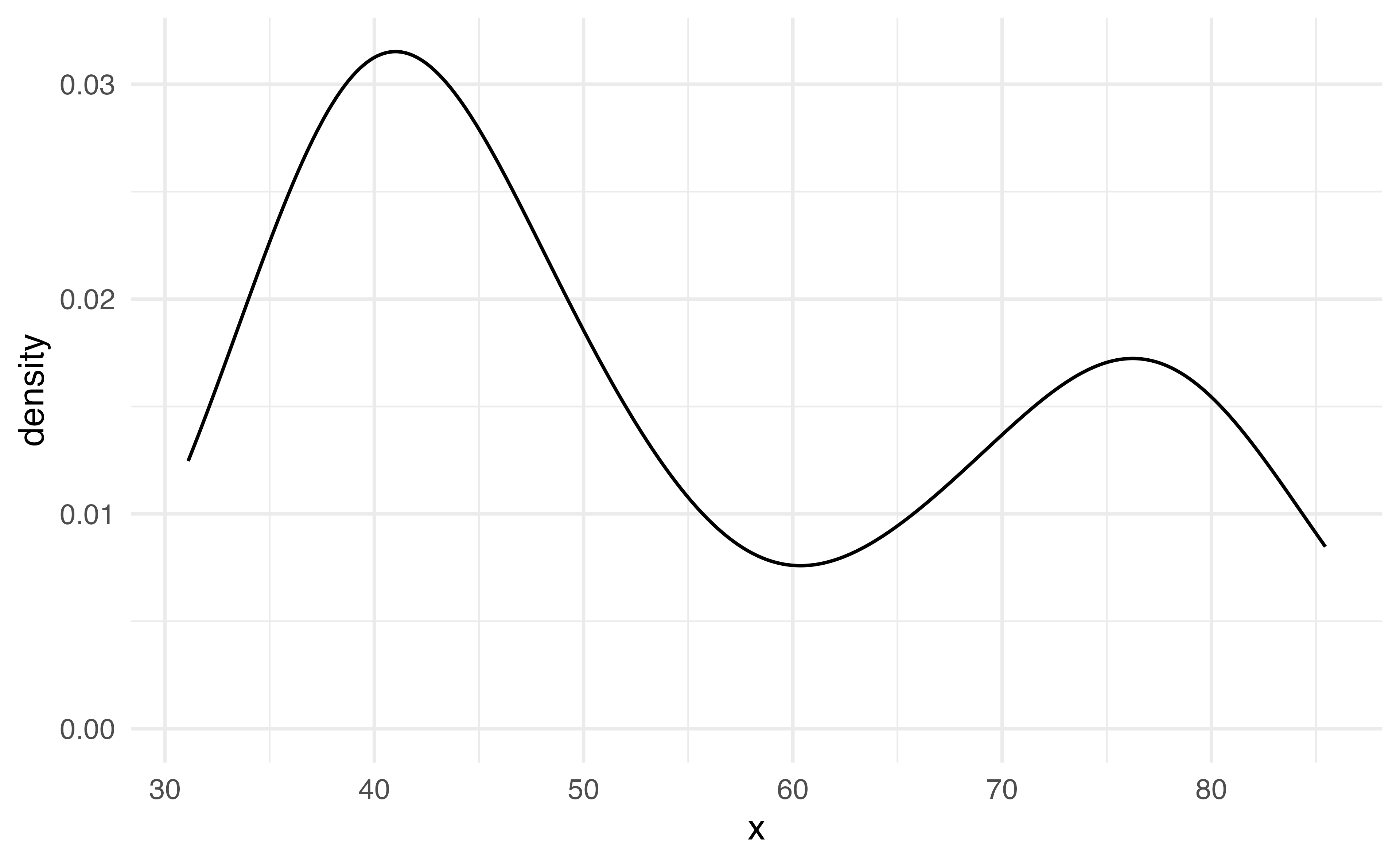
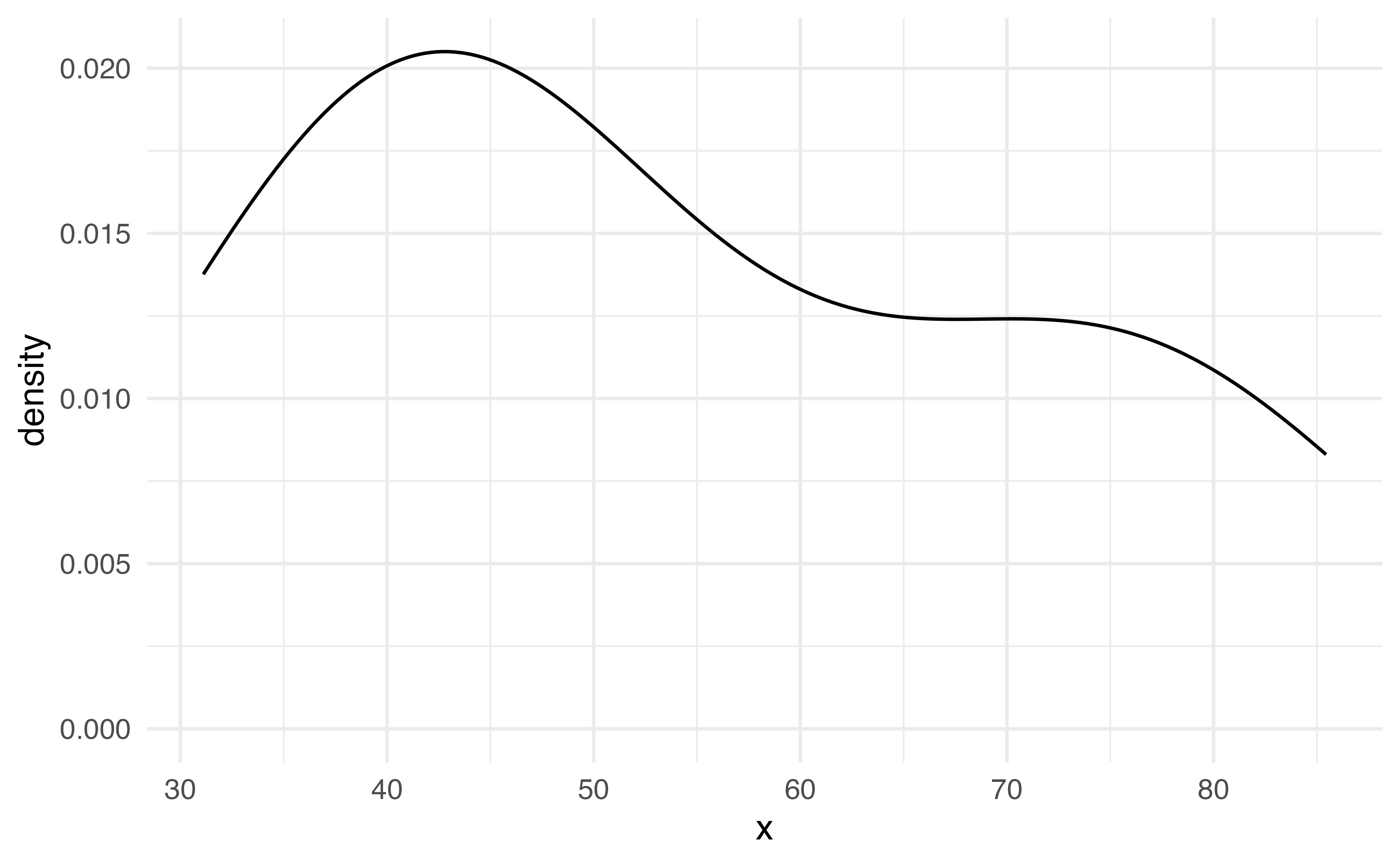
Density plots

Density plots
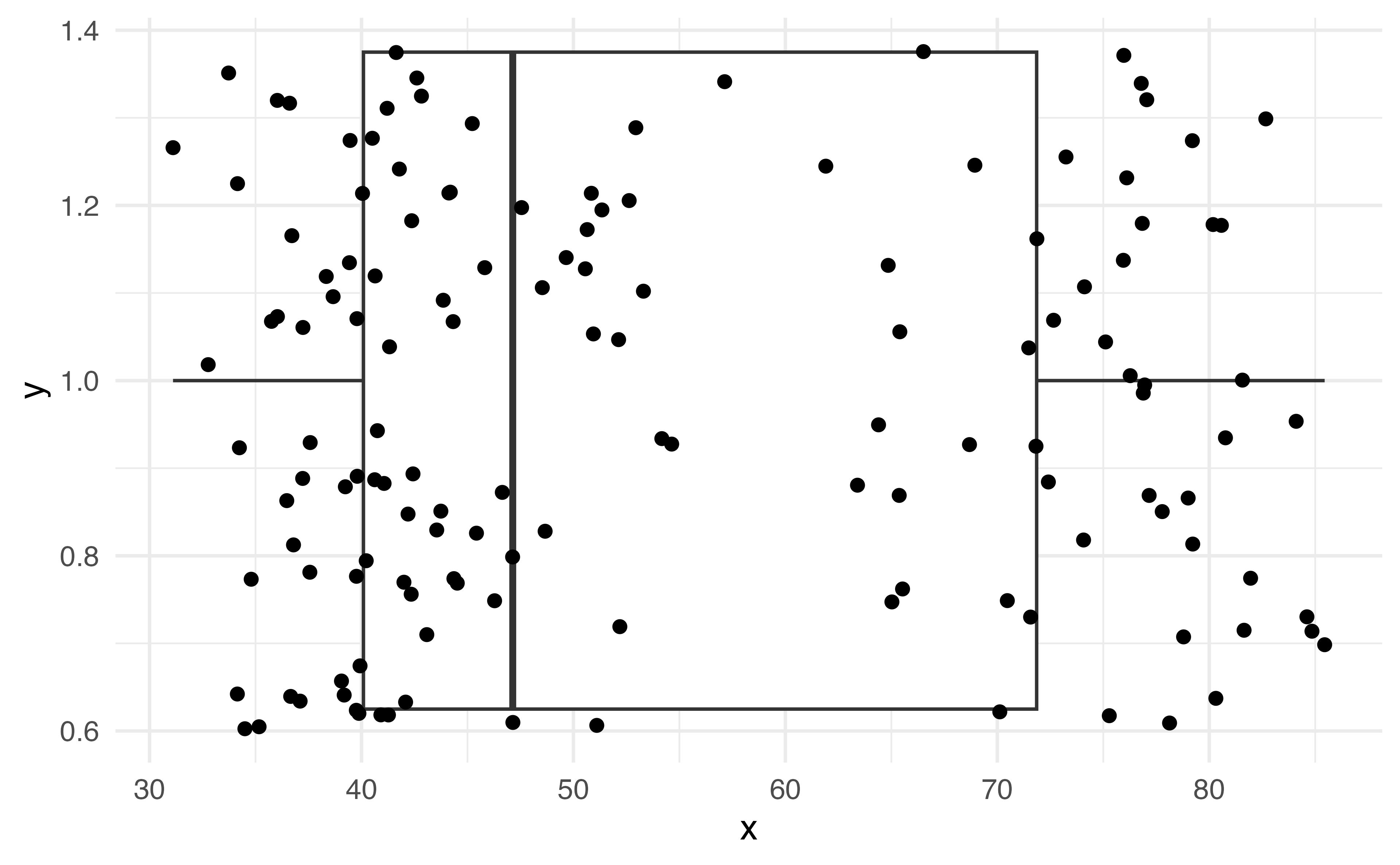
Boxplot
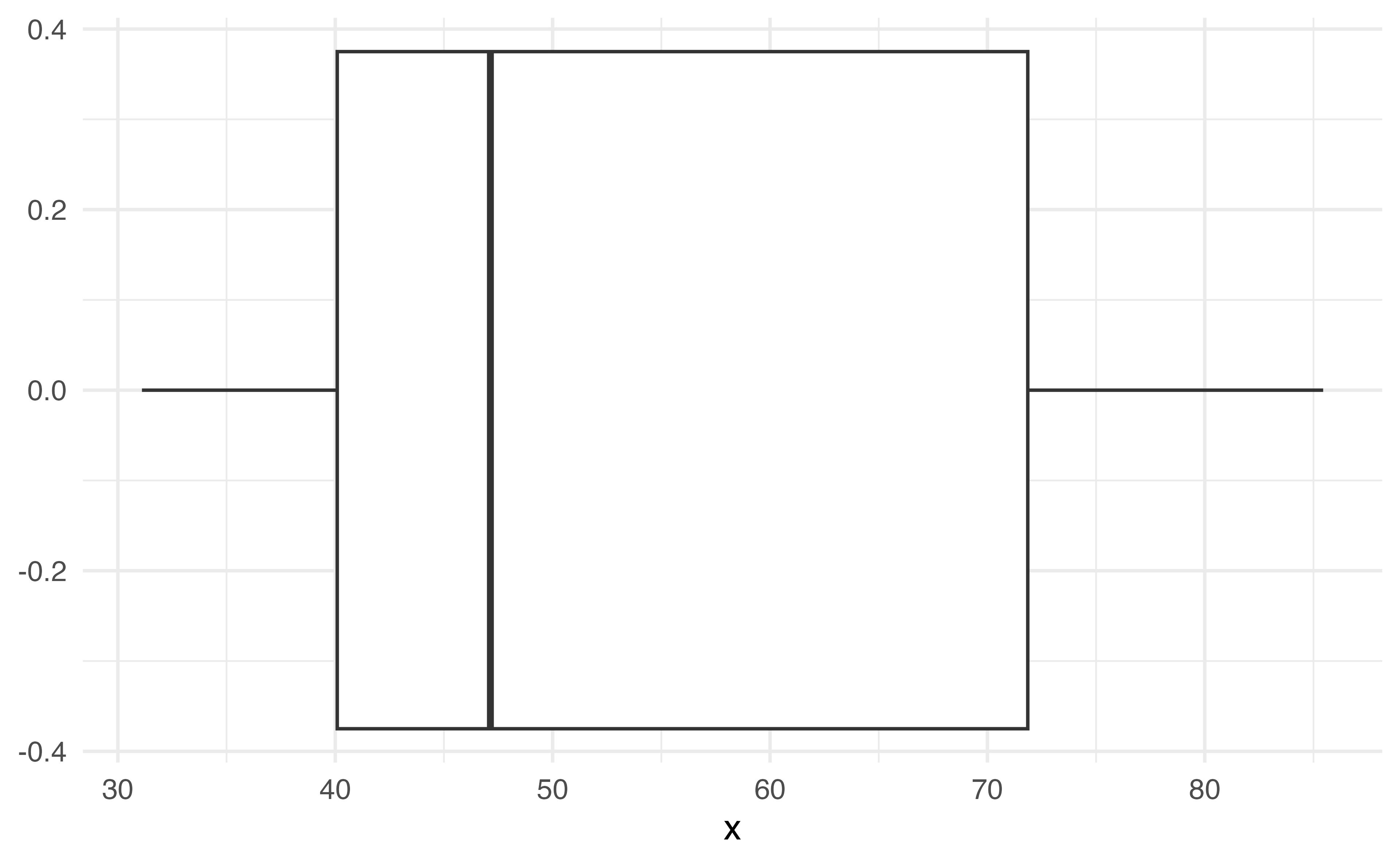
Does this give us as much information as the histogram?
00:30
Boxplot
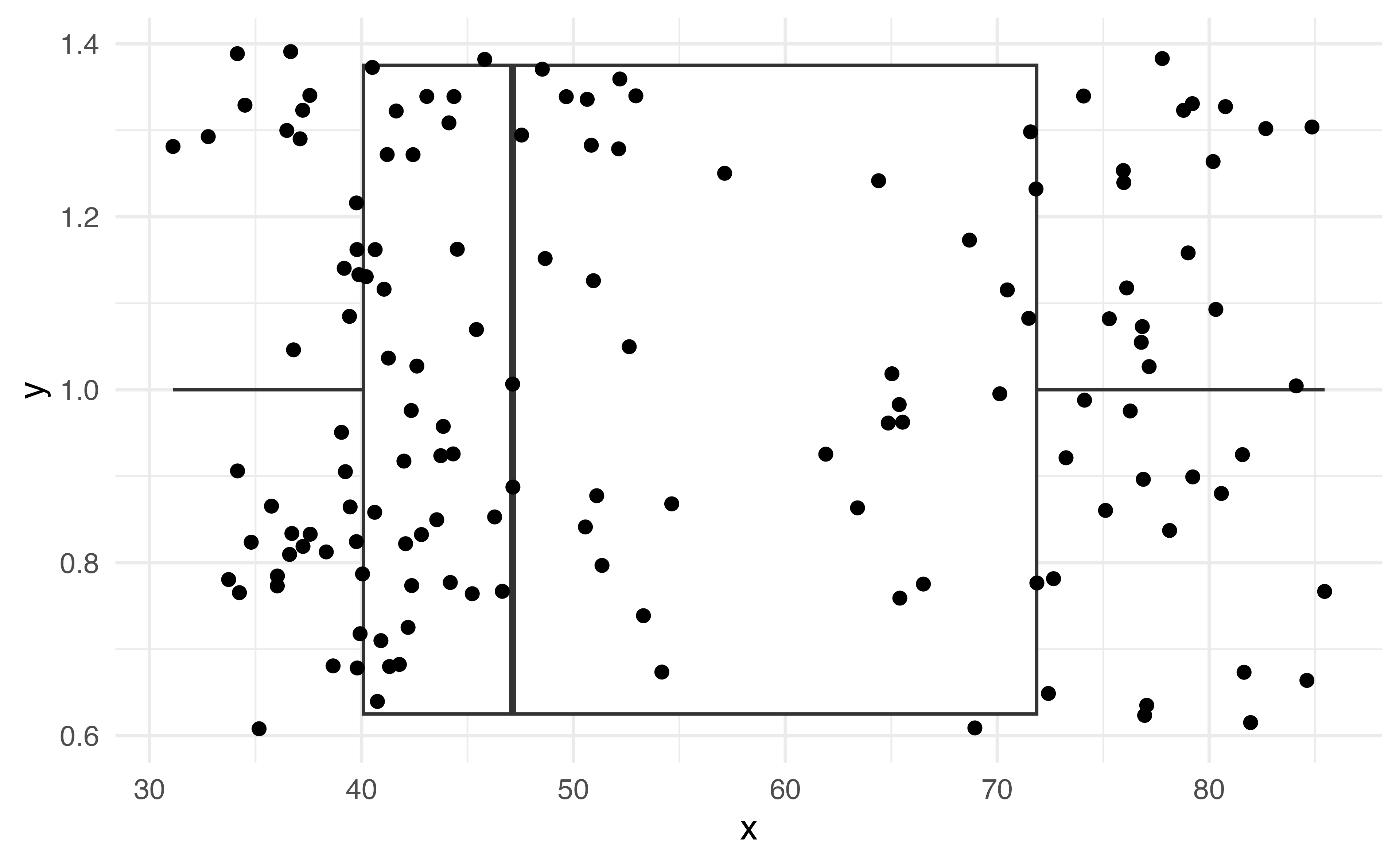
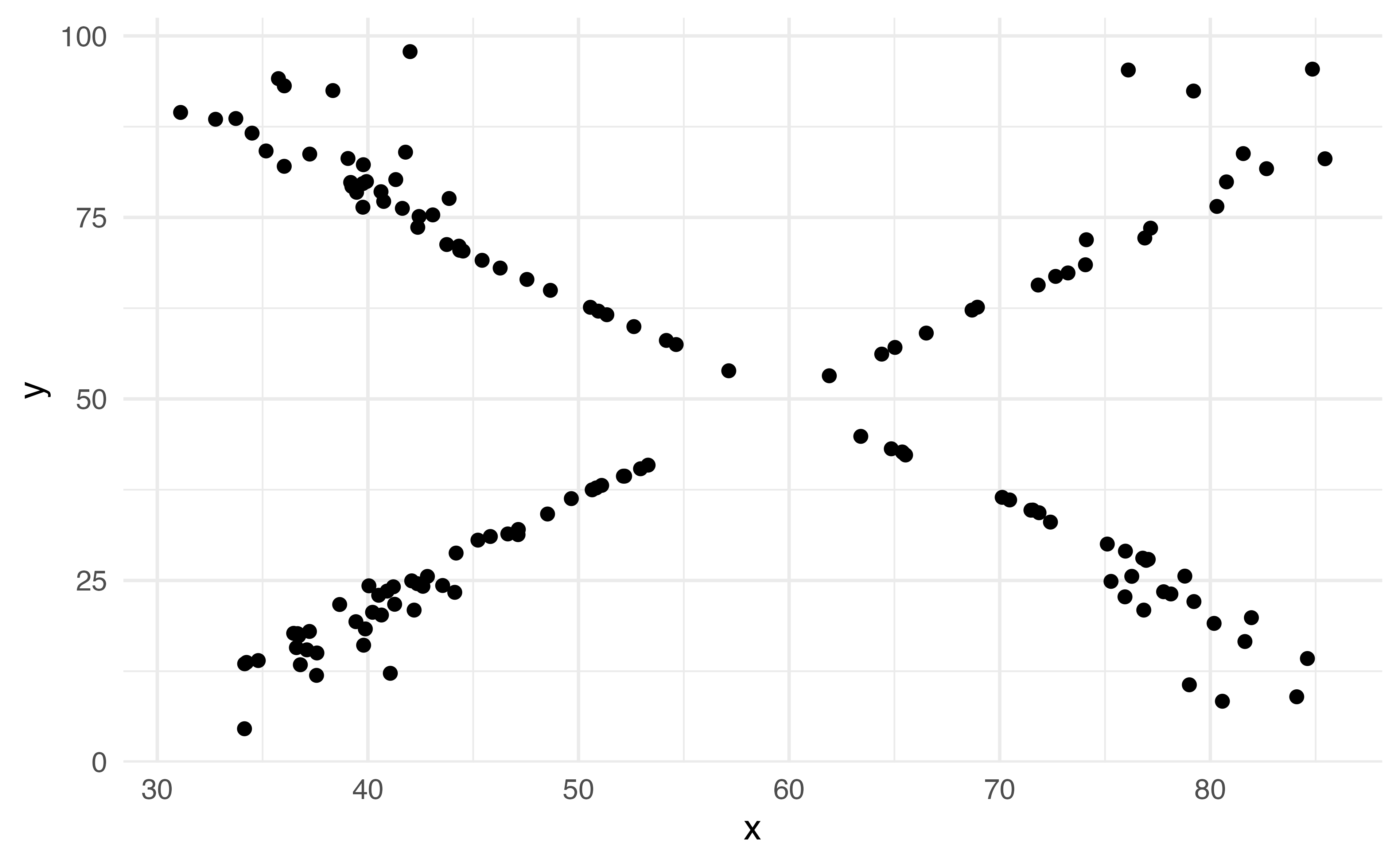
Always show your data!
Boxplot
Always show your data!
Scatterplot
Hex plot
Barplot
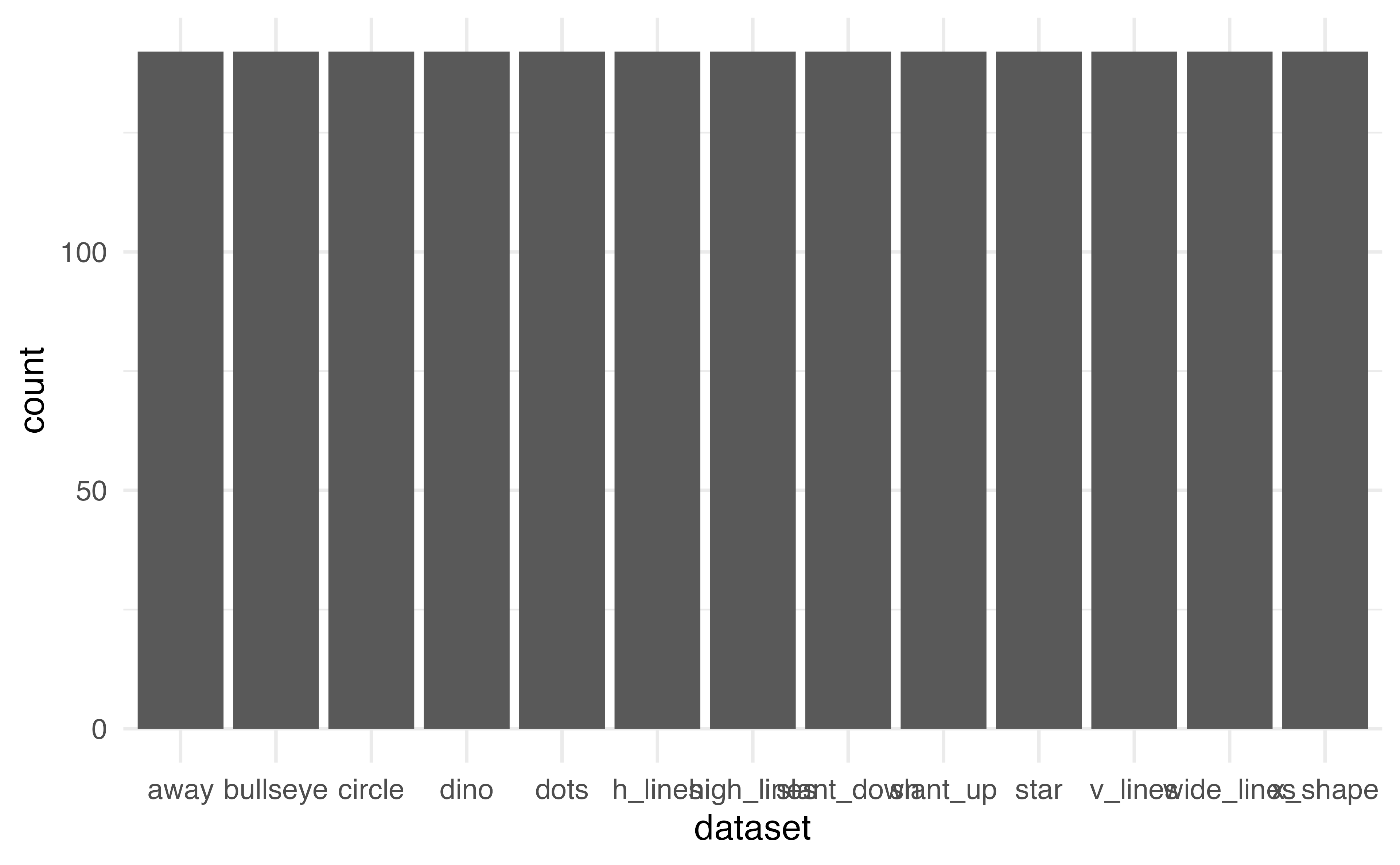
What does this plot tell us?
00:30
Barplot
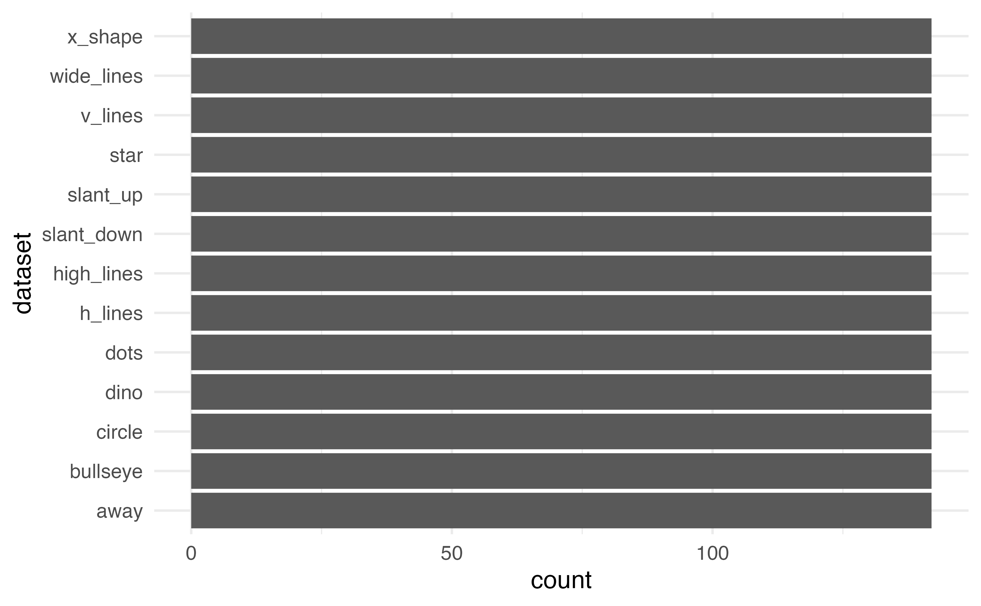
Flip the coordinates to make it easier to read
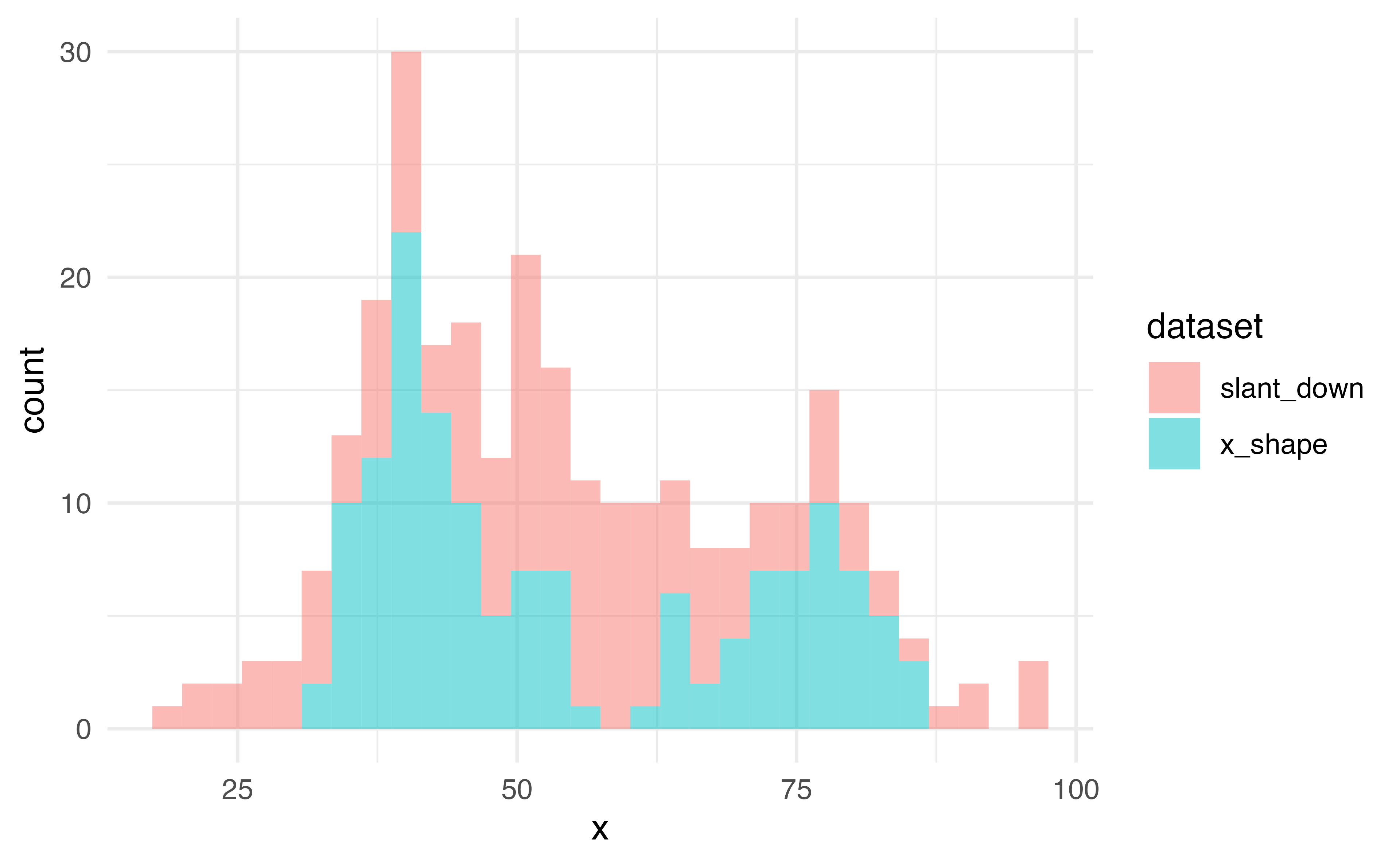
Histogram
Histogram
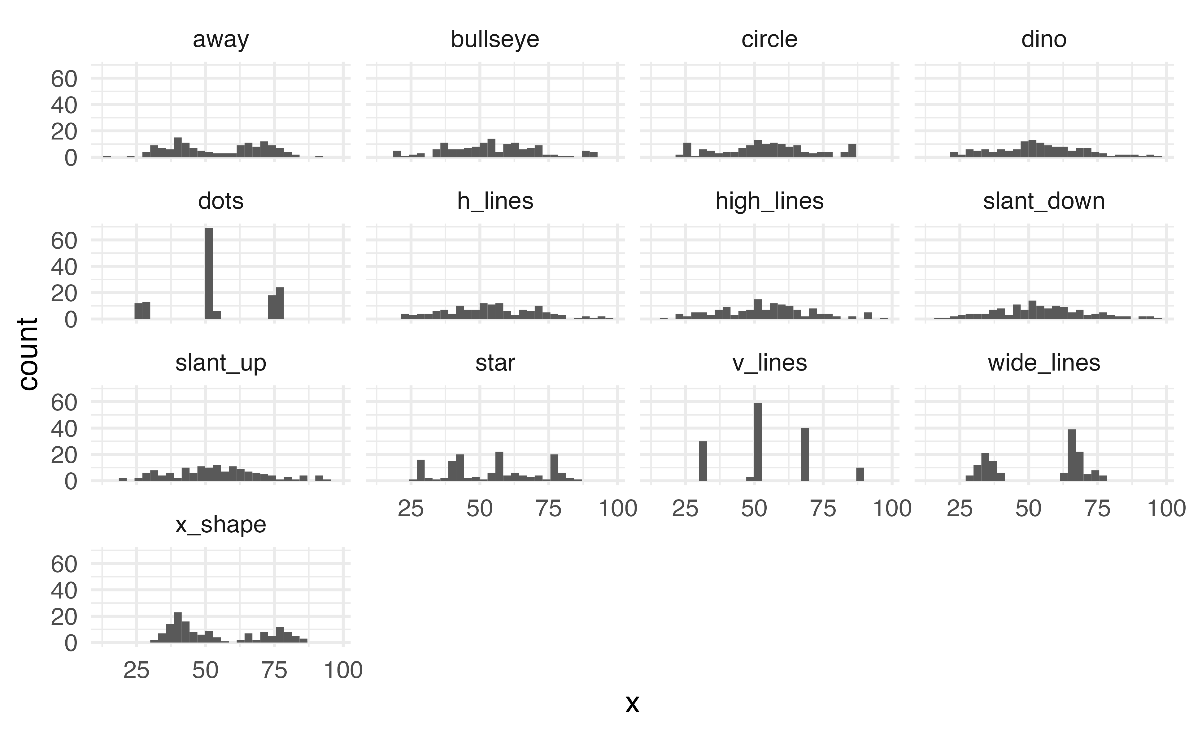
Histogram
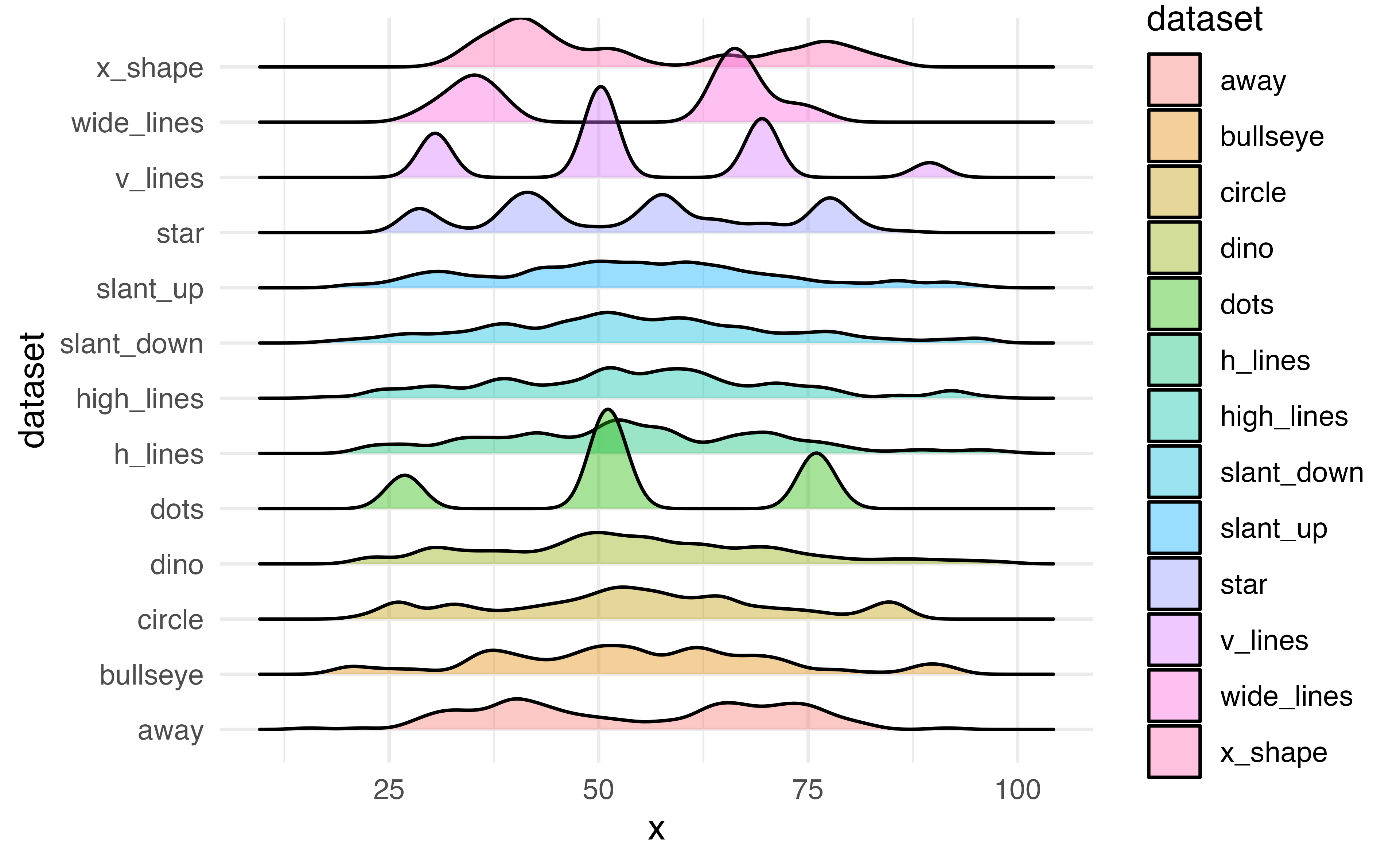
Ridge plots
Boxplot
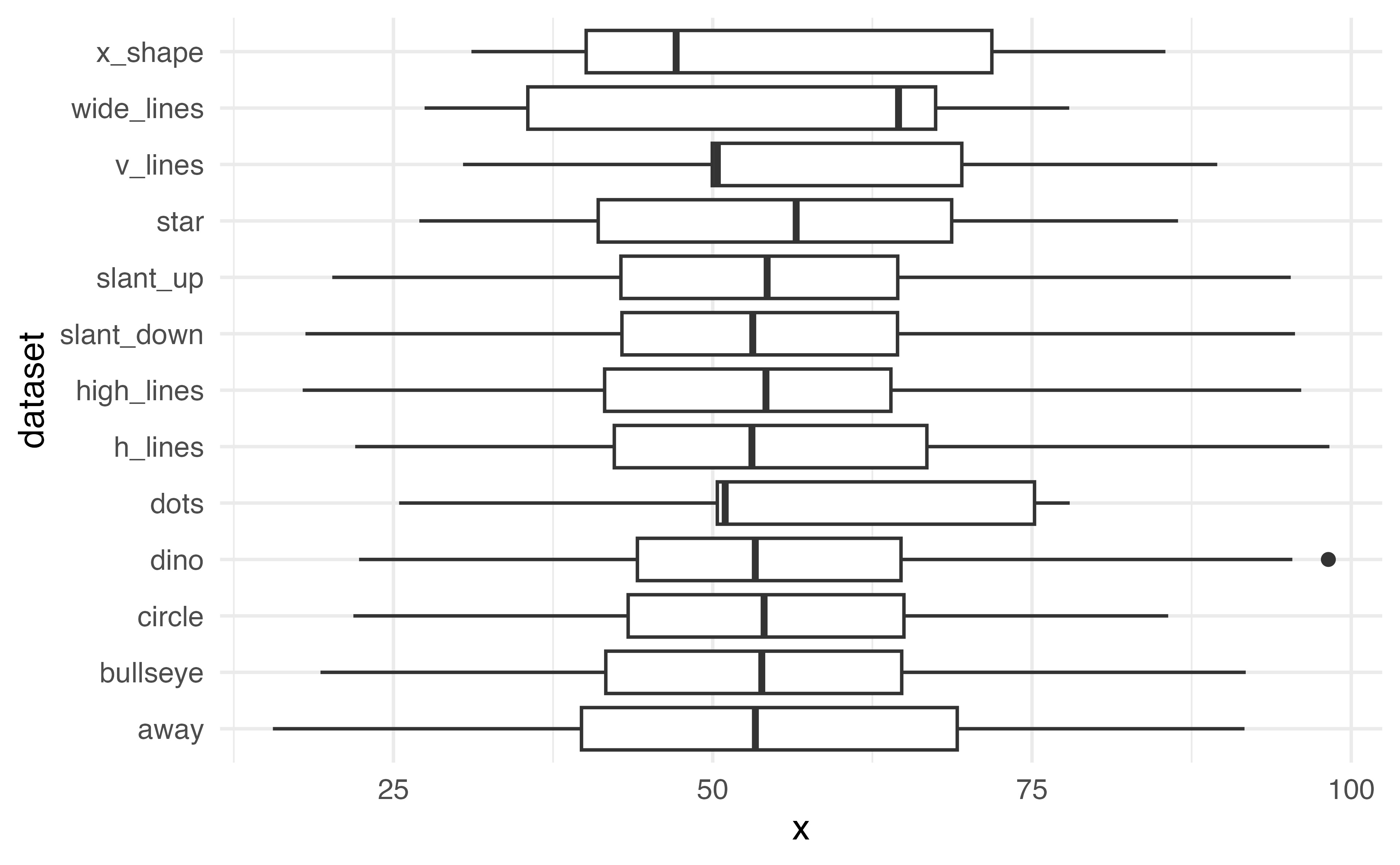
What is missing?
00:30
Boxplot
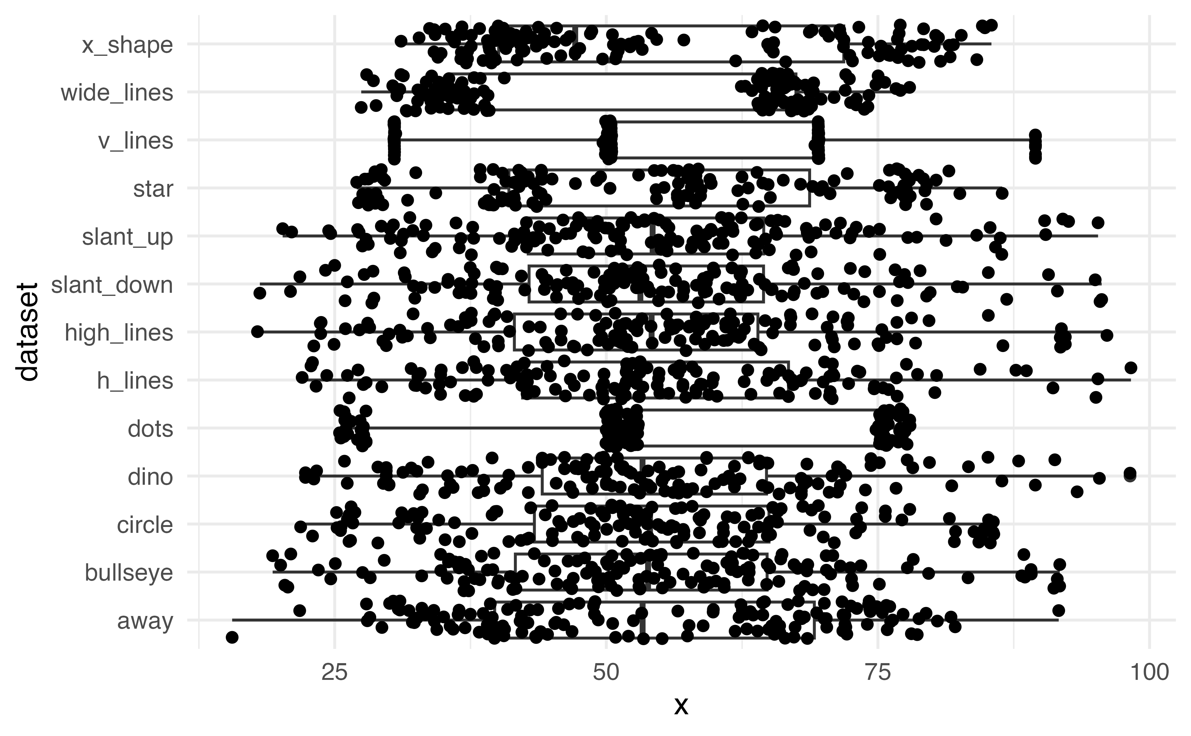
How can we make this more legible?
00:30
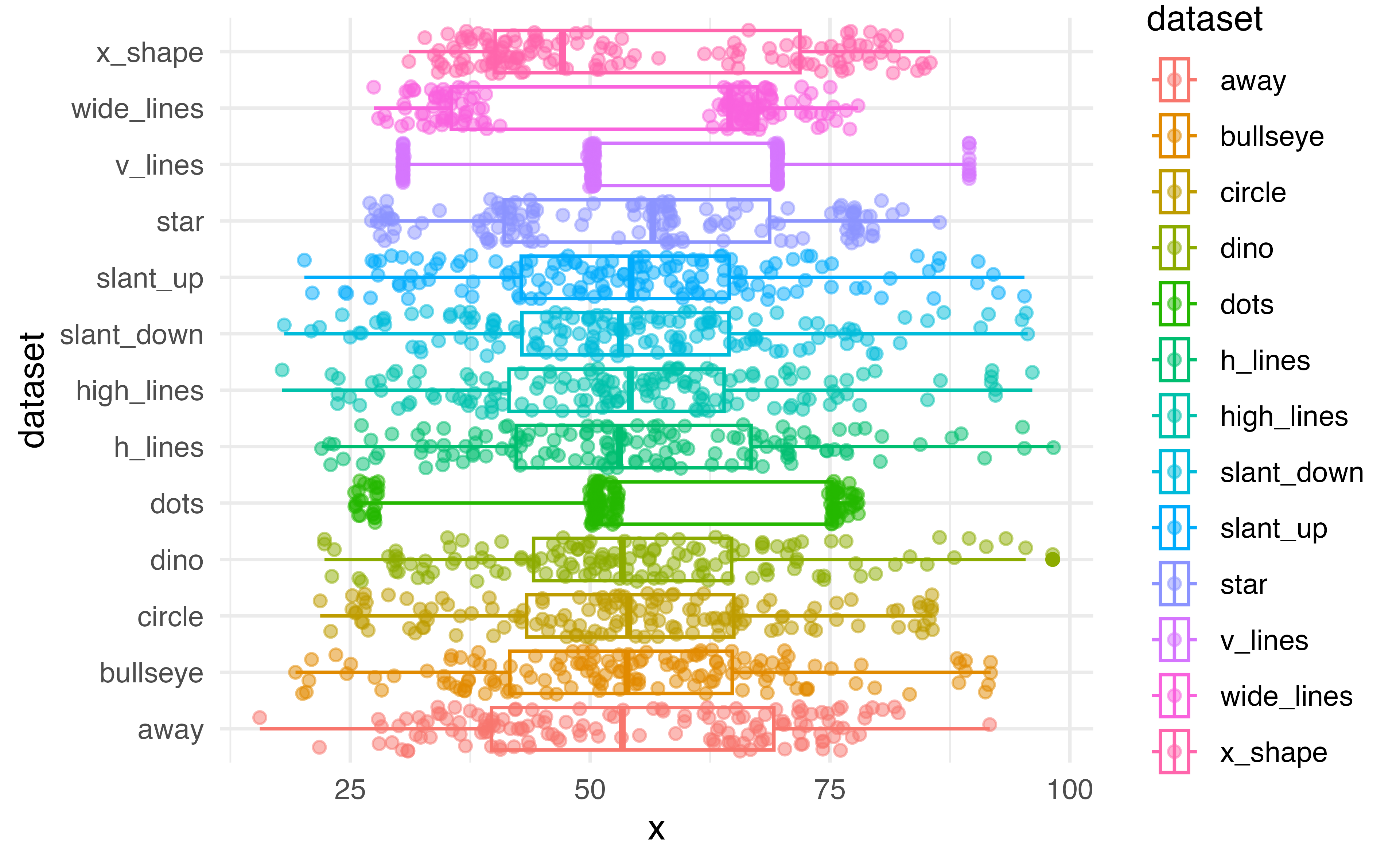
Boxplot
Application Exercise
Open the Welcome Penguins folder from the previous application exercise
Create a boxplot examining the relationship between the body mass of a penguin and their species.
Add jittered points to this plot
Add labels and a title to this plot
08:00