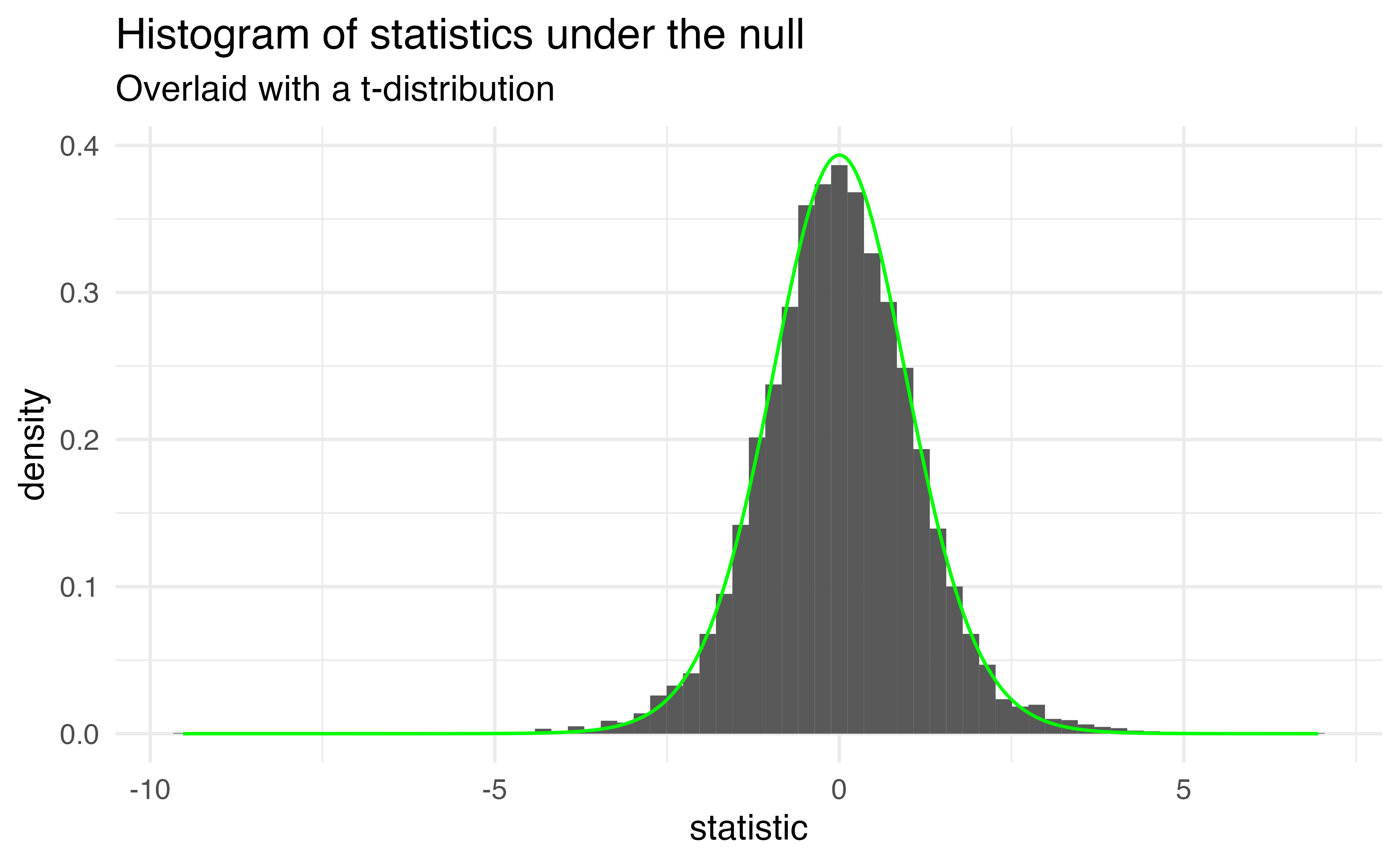
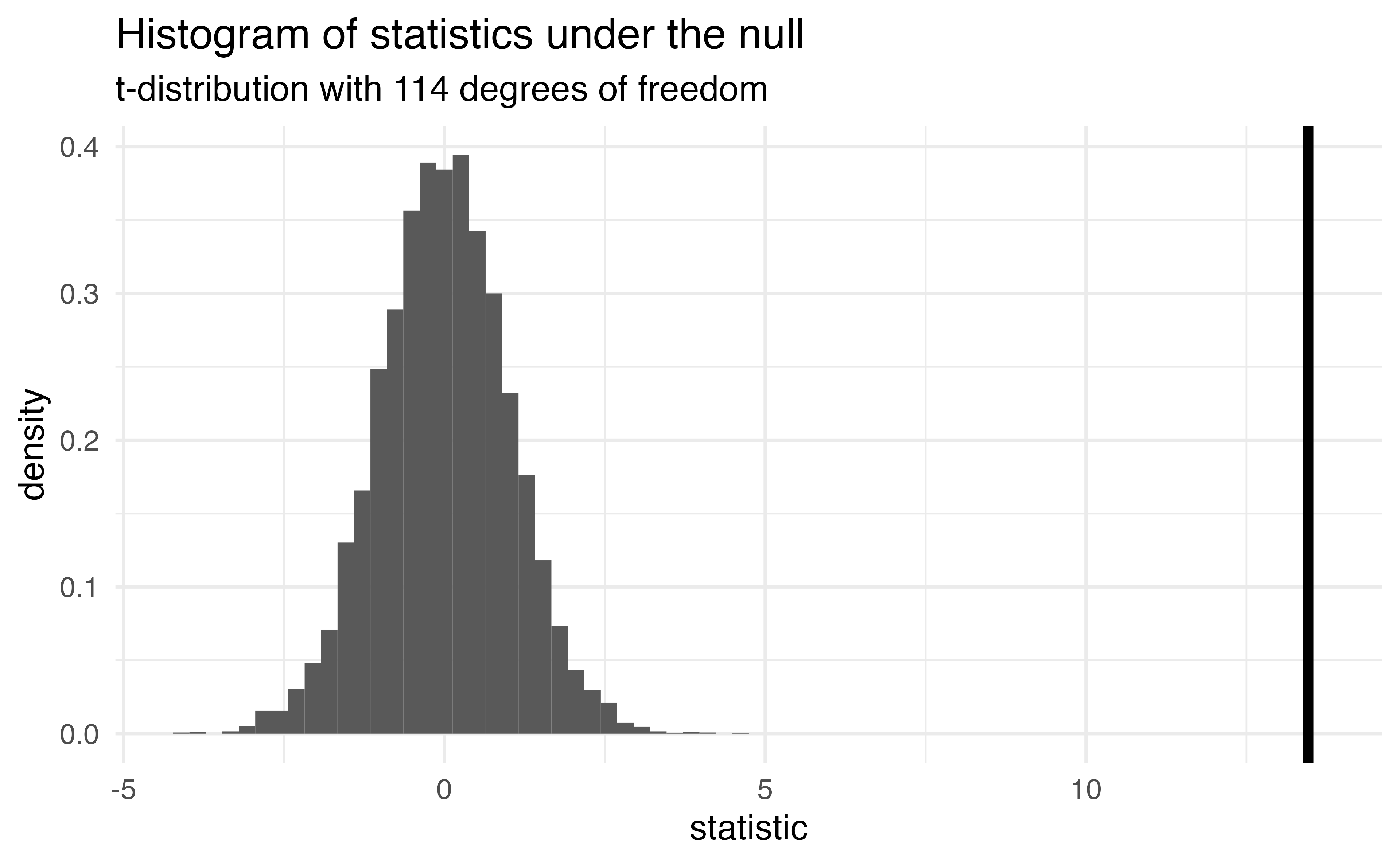
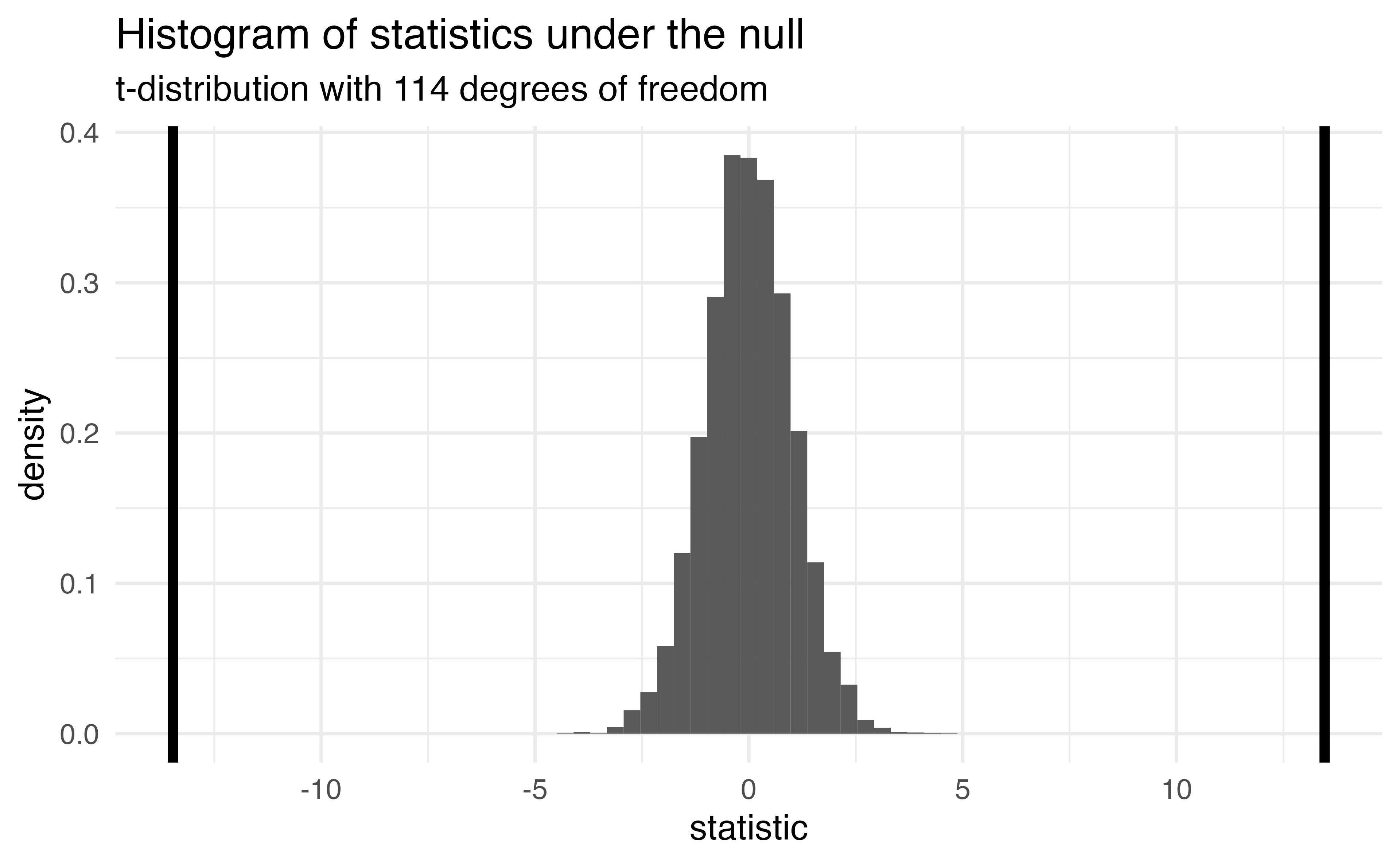
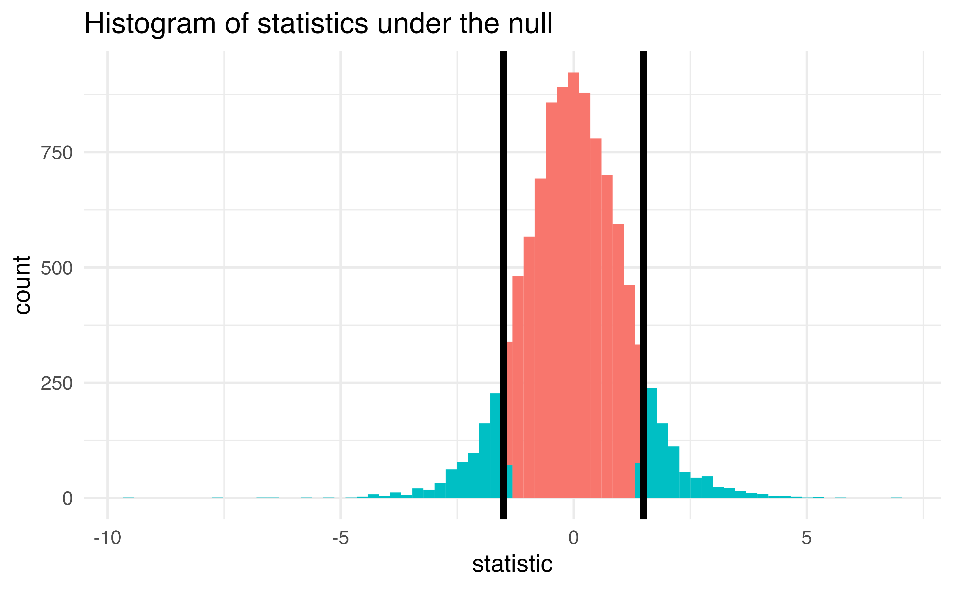
The proportion of area greater than 1.5 orless than -1.5.
pt(1.5, df =18, lower.tail =FALSE) *2
[1] 0.1509505
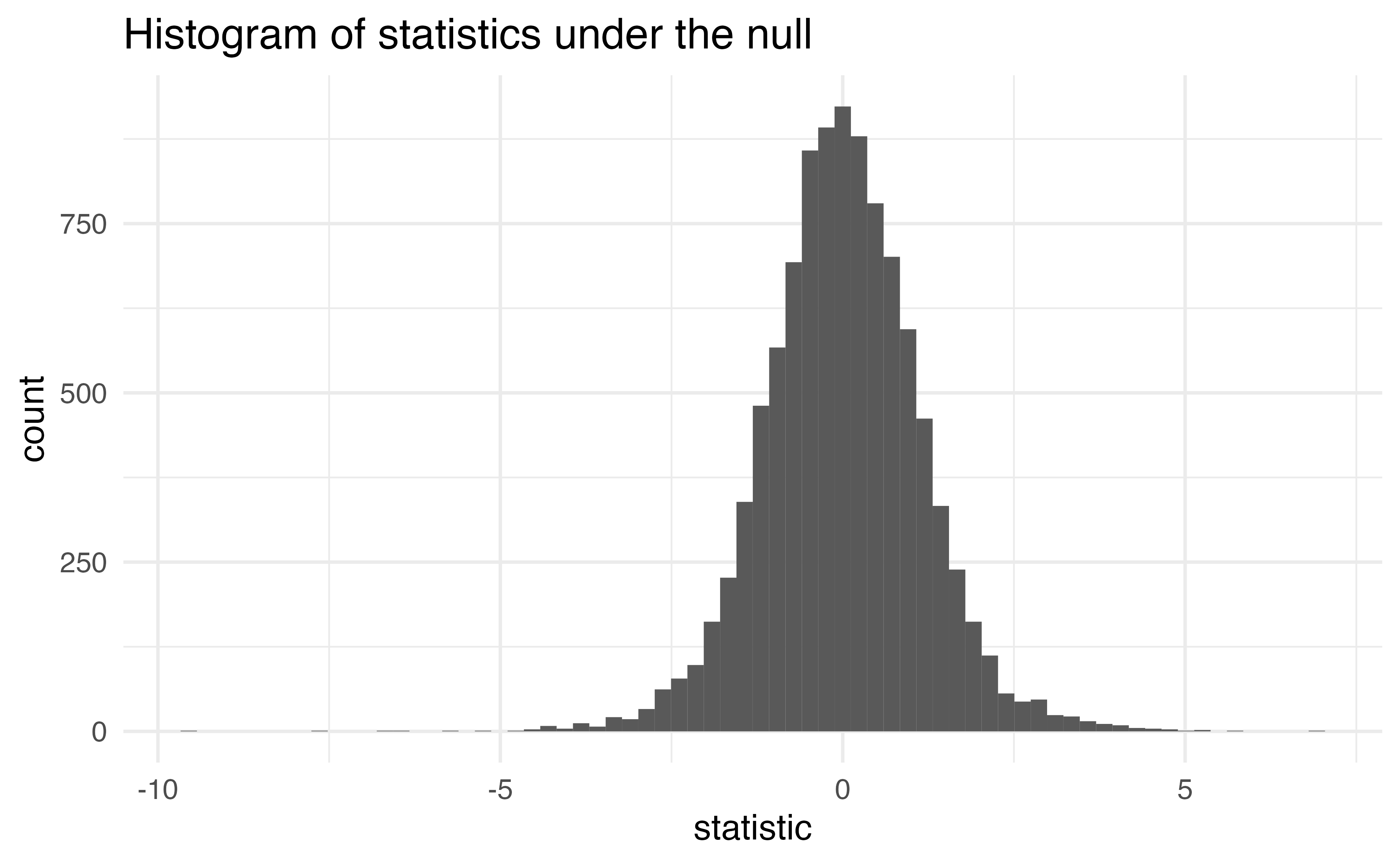
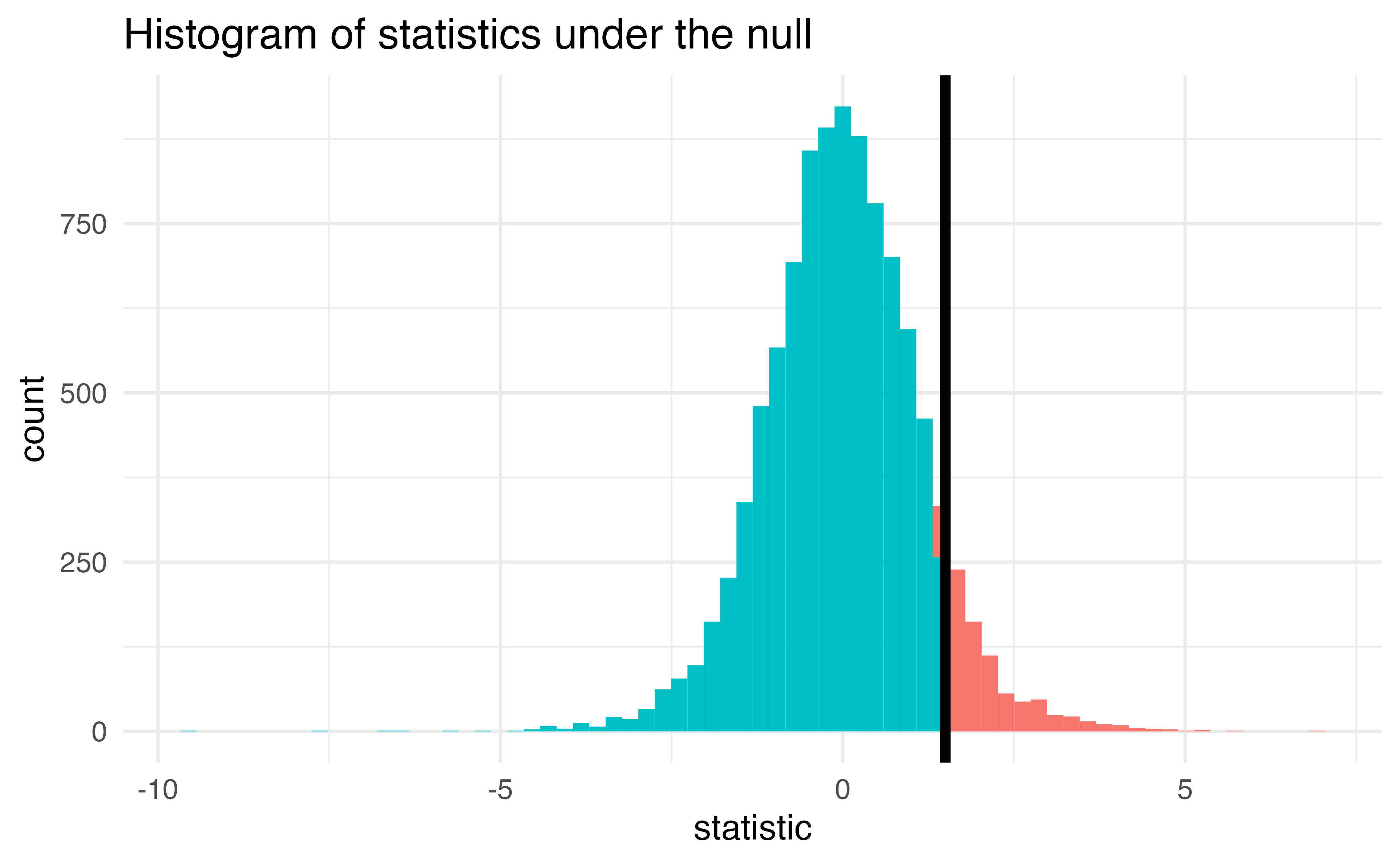
p-value
The probability of getting a statistic as extreme or more extreme than the observed test statistic given the null hypothesis is true
Hypothesis test
null hypothesis\(H_0: \beta_1 = 0\)
alternative hypothesis\(H_A: \beta_1 \ne 0\)
p-value: 0.15
Often, we have an \(\alpha\)-level cutoff to compare this to, for example 0.05. Since this is greater than 0.05, we fail to reject the null hypothesis
Application Exercise
Using the linear model you fit previously (mpg from wt and hp) - calculate the p-value for the coefficient for weight
Interpret this value. What is the null hypothesis? What is the alternative hypothesis? Do you reject the null?
04:00
confidence intervals
If we use the same sampling method to select different samples and computed an interval estimate for each sample, we would expect the true population parameter ( \(\beta_1\) ) to fall within the interval estimates 95% of the time.
If we use the same sampling method to select different samples and computed an interval estimate for each sample, we would expect the true population parameter ( \(\beta_1\) ) to fall within the interval estimates 95% of the time.
Linear Regression Questions
✔️ Is there a relationship between a response variable and predictors?
✔️ How strong is the relationship?
✔️ What is the uncertainty?
How accurately can we predict a future outcome?
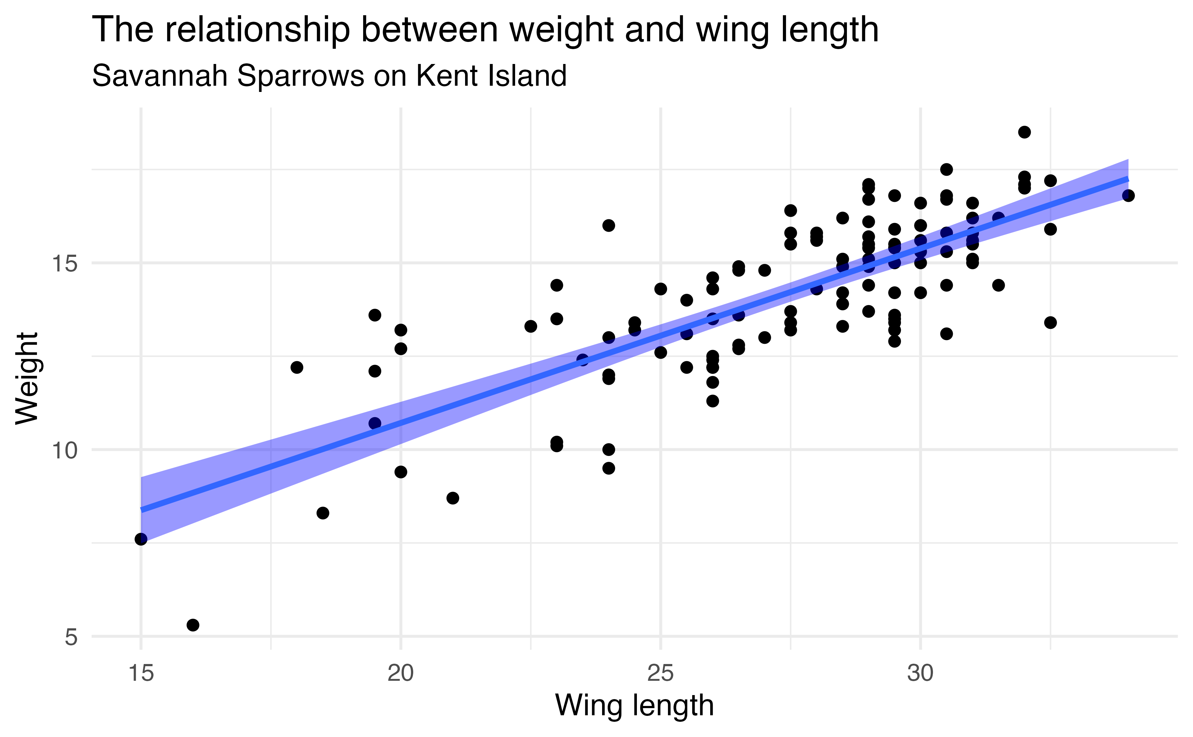
Sparrows
Using the information here, how could I predict a new sparrow’s weight if I knew the wing length was 30?
linear_reg() |>set_engine("lm") |>fit(Weight ~ WingLength, data = Sparrows) |>tidy()
Note: In previous classes, this may have been referred to as SSE (sum of squares error), the book uses RSS, so we will stick with that!
\[RSS = \sum(y_i - \hat{y}_i)^2\]
Linear Regression Accuracy
The total sum of squares represents the variability of the outcome, it is equivalent to the variability described by the model plus the remaining residual sum of squares
\[TSS = \sum(y_i - \bar{y})^2\]
Linear Regression Accuracy
There are many ways “model fit” can be assessed. Two common ones are:
# A tibble: 1 × 3
  .metric .estimator .estimate
  <chr>   <chr>          <dbl>
1 rsq     standard       0.614
Is this testing \(R^2\) or training \(R^2\)?
Application Exercise
Fit a linear model using the mtcars data frame predicting miles per gallon (mpg) from weight and horsepower (wt and hp), using polynomials with 4 degrees of freedom for both.
Estimate the training \(R^2\) using the rsq function.
Interpret this values.
04:00
Application Exercise
Create a cross validation object to do 5 fold cross validation using the mtcars data
Refit the model on this object (using fit_resamples)
Use collect_metrics to estimate the test \(R^2\) - how does this compare to the training \(R^2\) calculated in the previous exercise?
04:00
Additional Linear Regression Topics
Polynomial terms
Interactions
Outliers
Non-constant variance of error terms
High leverage points
Collinearity
Refer to Chapter 3 for more details on these topics if you need a refresher.