Non-linear relationships
What have we used so far to deal with non-linear relationships?
Hint: What did you use in Lab 02?
Polynomials!
Polynomials
\[y_i = \beta_0 + \beta_1x_i + \beta_2x_i^2+\beta_3x_i^3 \dots + \beta_dx_i^d+\epsilon_i\]
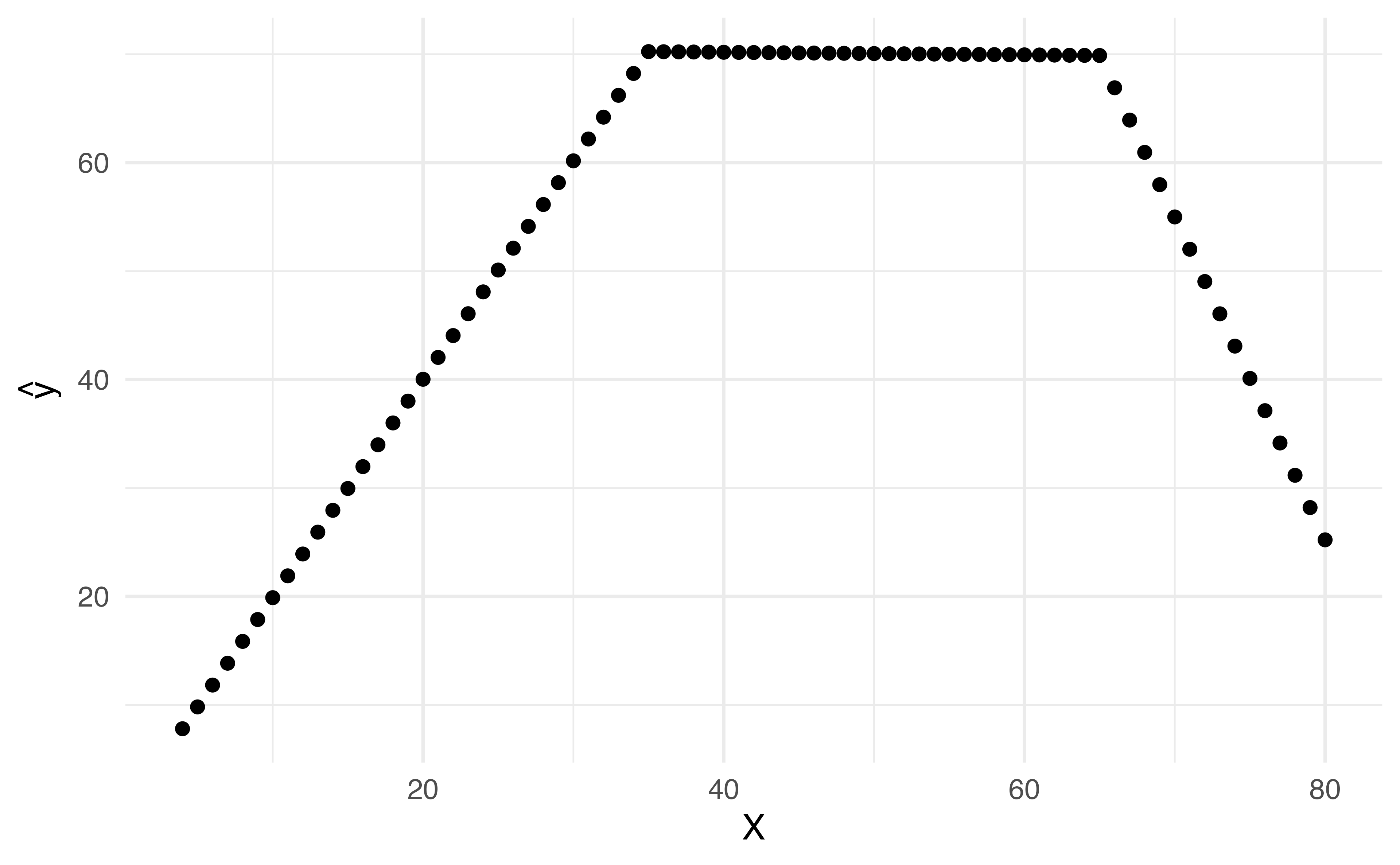
This is data from the Columbia World Fertility Survey (1975-76) to examine household compositions
Polynomials
\[y_i = \beta_0 + \beta_1x_i + \beta_2x_i^2+\beta_3x_i^3 \dots + \beta_dx_i^d+\epsilon_i\]
Fit here with a 4th degree polynomial
How is it done?
New variables are created ( \(X_1 = X\) , \(X_2 = X^2\) , \(X_3 = X^3\) , etc) and treated as multiple linear regression
We are not interested in the individual coefficients, we are interested in how a specific \(x\) value behaves
\(\hat{f}(x_0) = \hat\beta_0 + \hat\beta_1x_0 + \hat\beta_2x_0^2 + \hat\beta_3x_0^3 + \hat\beta_4x_0^4\) or more often a change between two values , \(a\) and \(b\) \(\hat{f}(b) -\hat{f}(a) = \hat\beta_1b + \hat\beta_2b^2 + \hat\beta_3b^3 + \hat\beta_4b^4 - \hat\beta_1a - \hat\beta_2a^2 - \hat\beta_3a^3 -\hat\beta_4a^4\) \(\hat{f}(b) -\hat{f}(a) =\hat\beta_1(b-a) + \hat\beta_2(b^2-a^2)+\hat\beta_3(b^3-a^3)+\hat\beta_4(b^4-a^4)\)
Polynomial Regression
\[\hat{f}(b) -\hat{f}(a) =\hat\beta_1(b-a) + \hat\beta_2(b^2-a^2)+\hat\beta_3(b^3-a^3)+\hat\beta_4(b^4-a^4)\]
How do you pick \(a\) and \(b\) ?
If given no other information, a sensible choice may be the 25th and 75th percentiles of \(x\)
Polynomial Regression
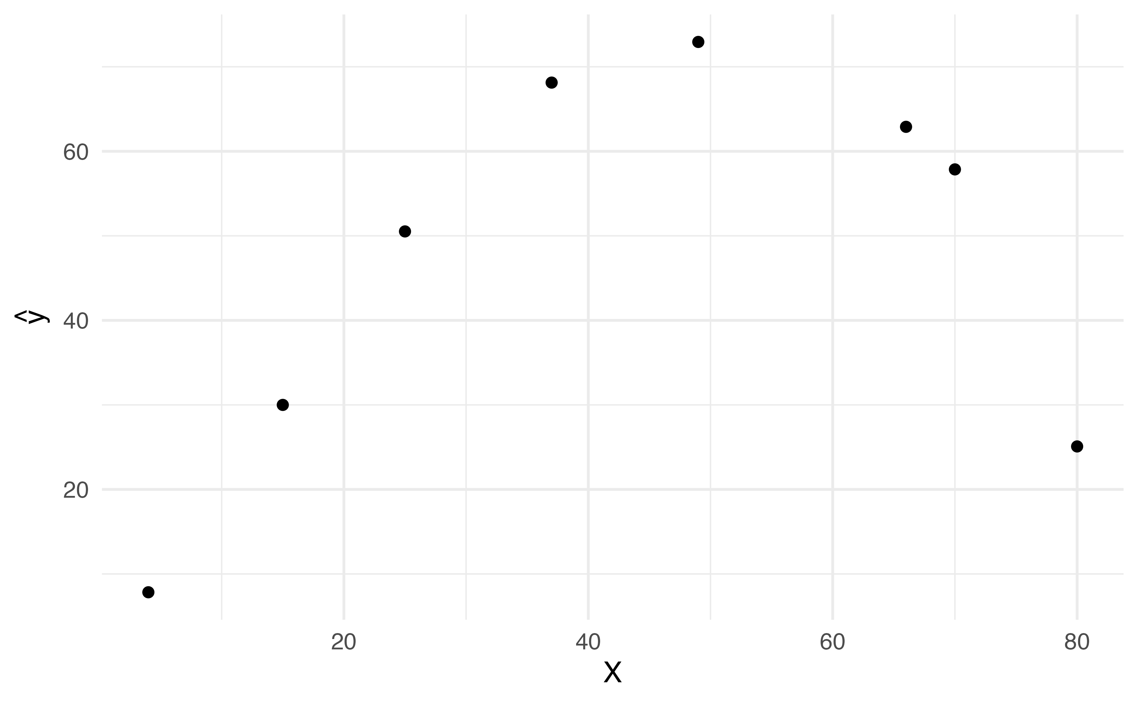
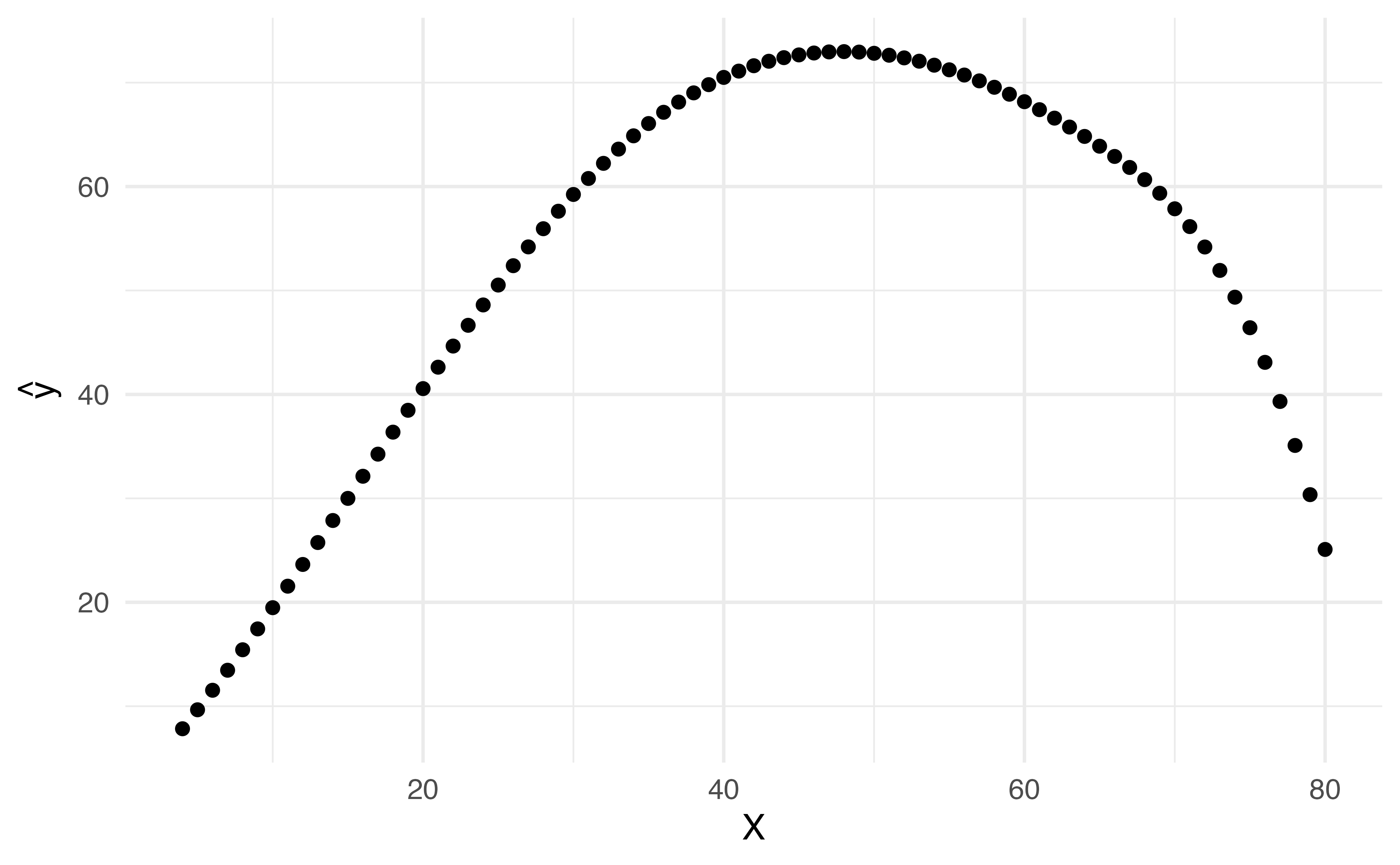
Application Exercise\[pop = \beta_0 + \beta_1age + \beta_2age^2 + \beta_3age^3 +\beta_4age^4+ \epsilon\]
Using the information below, write out the equation to predicted change in population from a change in age from the 25th percentile (24.5) to a 75th percentile (73.5).
(Intercept)
1672.0854
64.5606
25.8995
0.0000
age
-10.6429
9.2268
-1.1535
0.2516
I(age^2)
-1.1427
0.3857
-2.9627
0.0039
I(age^3)
0.0216
0.0059
3.6498
0.0004
I(age^4)
-0.0001
0.0000
-3.6540
0.0004
Choosing \(d\)
\[y_i = \beta_0 + \beta_1x_i + \beta_2x_i^2+\beta_3x_i^3 \dots + \beta_dx_i^d+\epsilon_i\]
Either:
Pre-specify \(d\) (before looking 👀 at your data!)
Use cross-validation to pick \(d\)
Polynomial Regression
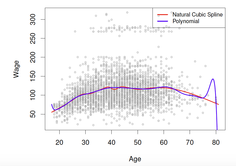
Polynomials have notoriously bad tail behavior (so they can be bad for extrapolation)
Step functions
Another way to create a transformation is to cut the variable into distinct regions
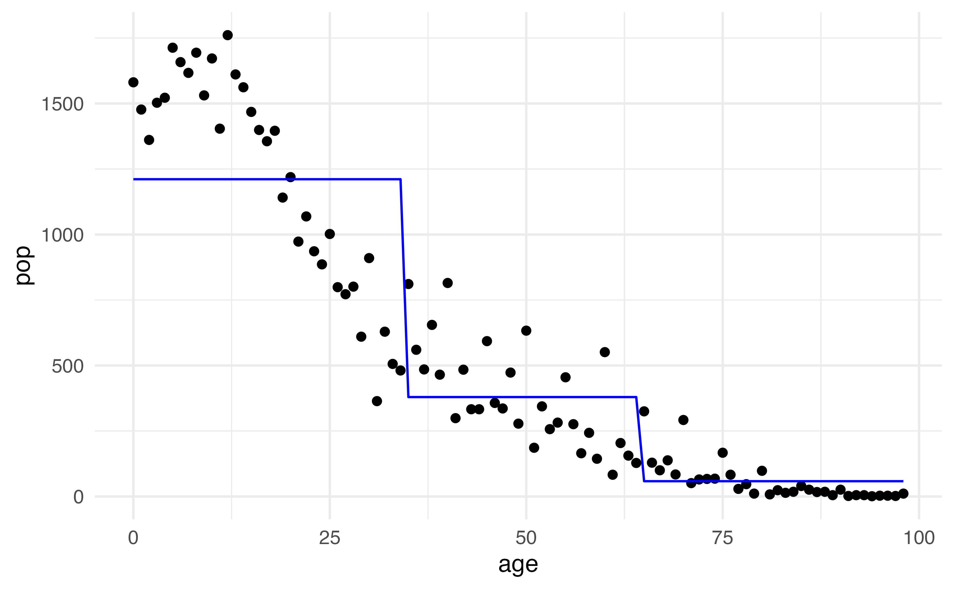
\[C_1(X) = I(X < 35), C_2(X) = I(35\leq X<65), C_3(X) = I(X \geq 65)\]
Step functions
Create dummy variables for each group
Include each of these variables in multiple regression
The choice of cutpoints or knots can be problematic (and make a big difference!)
Step functions
\[C_1(X) = I(X < 35), C_2(X) = I(35\leq X<65), C_3(X) = I(X \geq 65)\]
What is the predicted value when \(age = 25\) ?
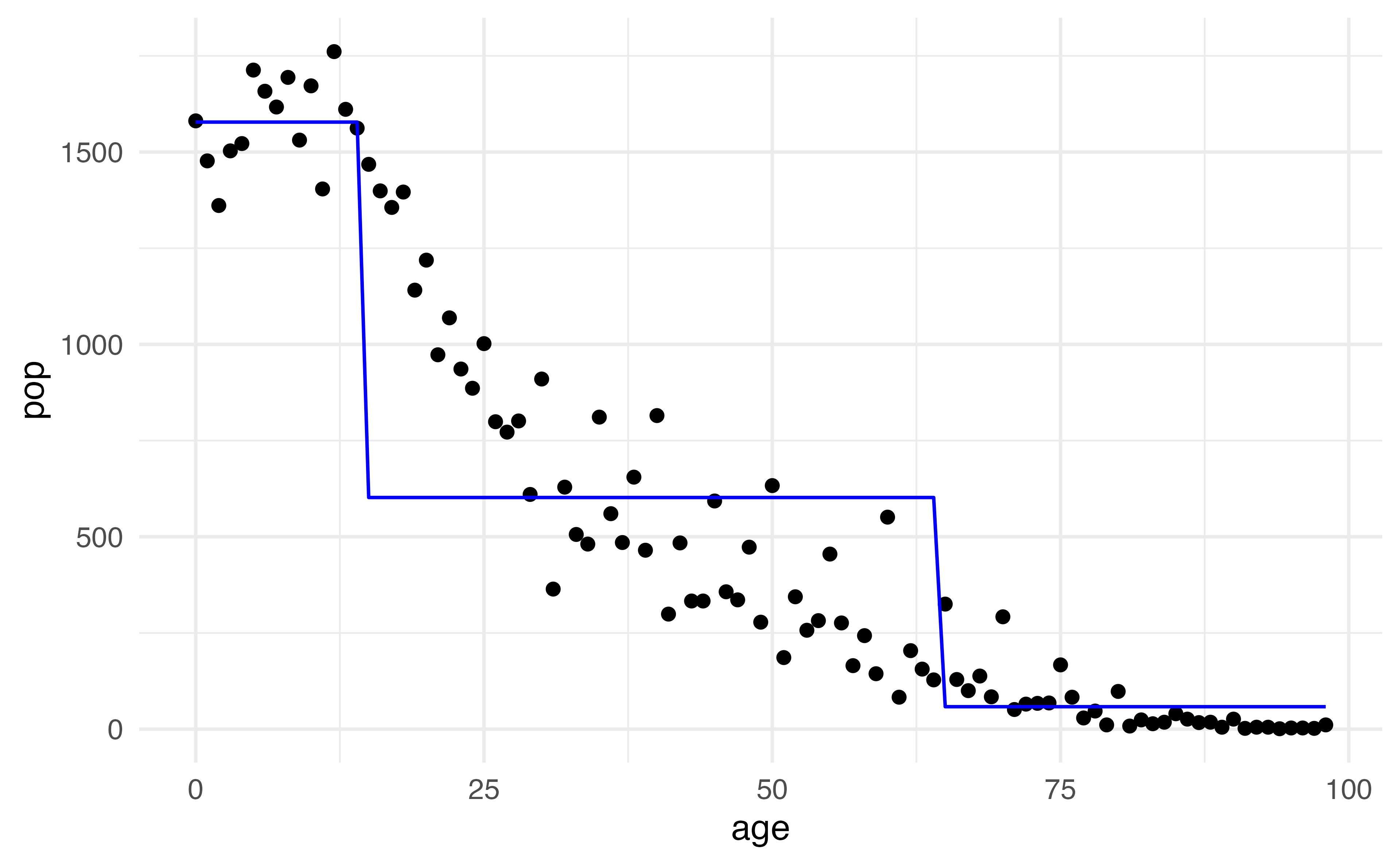
Step functions
\[C_1(X) = I(X < 15), C_2(X) = I(15\leq X<65), C_3(X) = I(X \geq 65)\]
What is the predicted value when \(age = 25\) ?
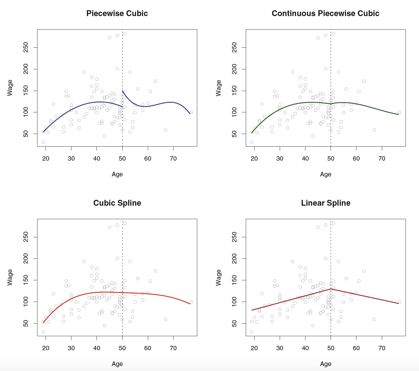
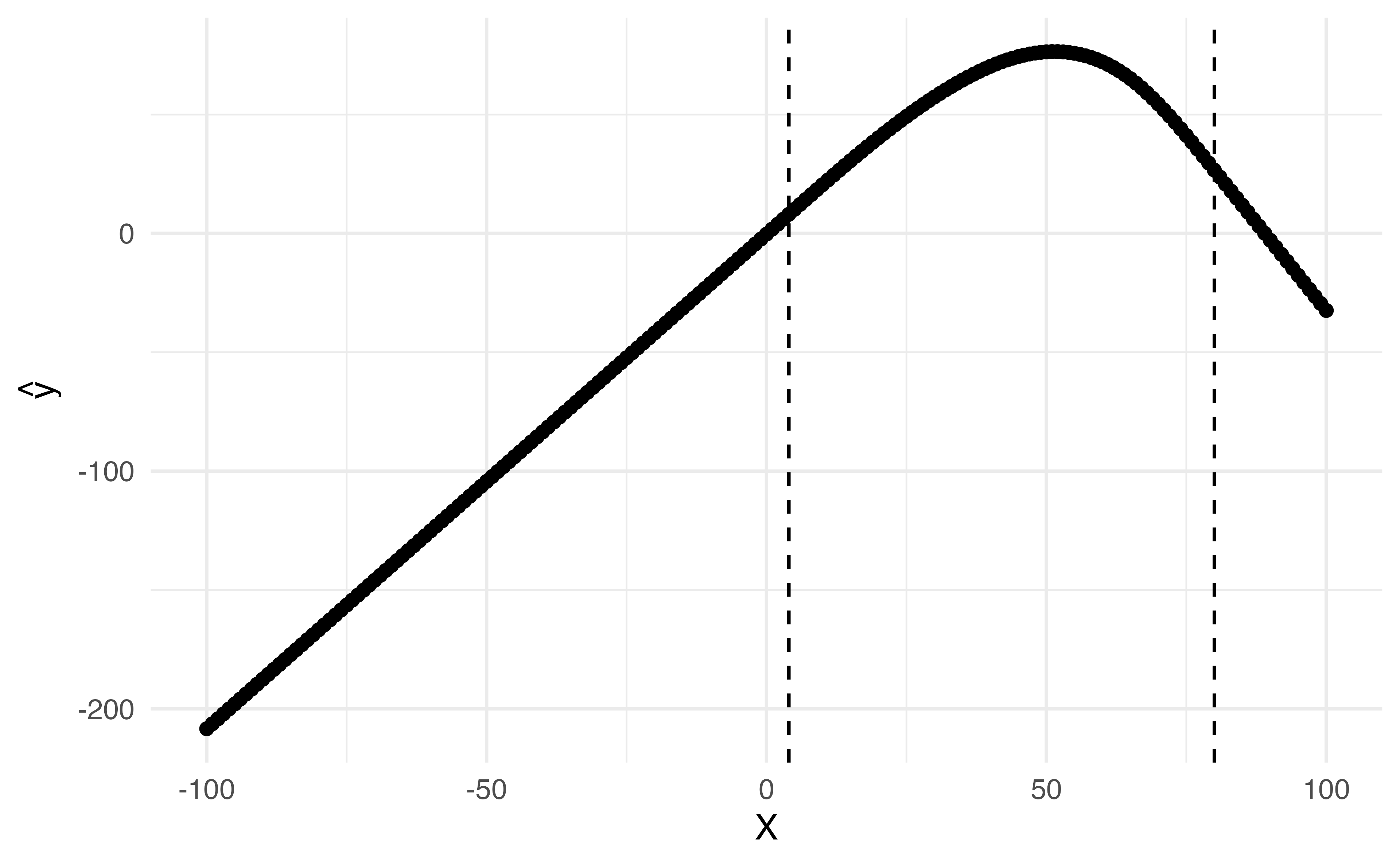
Piecewise polynomials
Instead of a single polynomial in \(X\) over it’s whole domain, we can use different polynomials in regions defined by knots
\[y_i = \begin{cases}\beta_{01}+\beta_{11}x_i + \beta_{21}x^2_i+\beta_{31}x^3_i+\epsilon_i& \textrm{if } x_i < c\\ \beta_{02}+\beta_{12}x_i + \beta_{22}x_i^2 + \beta_{32}x_{i}^3+\epsilon_i&\textrm{if }x_i\geq c\end{cases}\]
What could go wrong here?
It would be nice to have constraints (like continuity!)
Insert splines!
Linear Splines
A linear spline with knots at \(\xi_k\) , \(k = 1,\dots, K\) is a piecewise linear polynomial continuous at each knot
\[y_i = \beta_0 + \beta_1b_1(x_i)+\beta_2b_2(x_i)+\dots+\beta_{K+1}b_{K+1}(x_i)+\epsilon_i\]
\(b_k\) are basis functions \(\begin{align}b_1(x_i)&=x_i\\ b_{k+1}(x_i)&=(x_i-\xi_k)_+,k=1,\dots,K\end{align}\) Here \(()_+\) means the positive part
\((x_i-\xi_k)_+=\begin{cases}x_i-\xi_k & \textrm{if } x_i>\xi_k\\0&\textrm{otherwise}\end{cases}\)
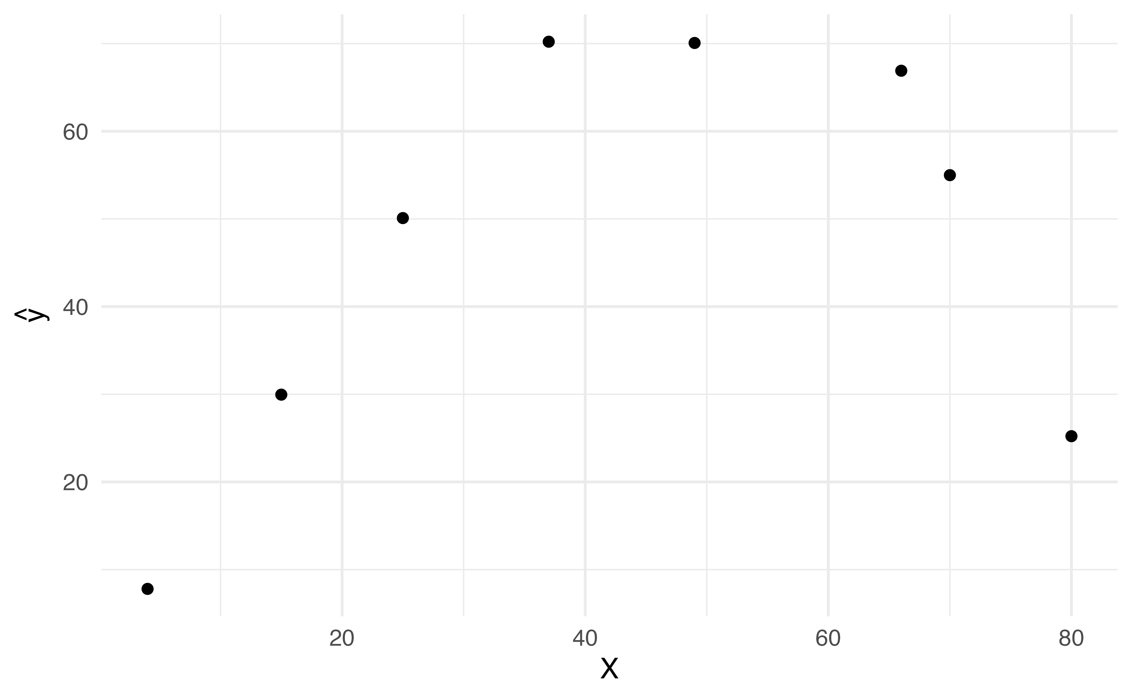
Application ExerciseLet’s create data set to fit a linear spline with 2 knots: 35 and 65.
Using the data to the left create a new dataset with three variables: \(b_1(x), b_2(x), b_3(x)\)
Write out the equation you would be fitting to estimate the effect on some outcome \(y\) using this linear spline
Linear Spline
➡️
4
0
0
15
0
0
25
0
0
37
2
0
49
14
0
66
31
1
70
35
5
80
45
15
Application ExerciseBelow is a linear regression model fit to include the 3 bases you just created with 2 knots: 35 and 65. Use the information here to draw the relationship between \(x\) and \(y\) .
(Intercept)
-0.3
0.2
-1.3
0.3
b1
2.0
0.0
231.3
0.0
b2
-2.0
0.0
-130.0
0.0
b3
-3.0
0.0
-116.5
0.0
Linear Splines
4
0
0
15
0
0
25
0
0
37
2
0
49
14
0
66
31
1
70
35
5
80
45
15
Linear Splines
Linear Splines
Cubic Splines
A cubic splines with knots at \(\xi_i, k = 1, \dots, K\) is a piecewise cubic polynomial with continuous derivatives up to order 2 at each knot.
Again we can represent this model with truncated power functions
\[y_i = \beta_0 + \beta_1b_1(x_i)+\beta_2b_2(x_i)+\dots+\beta_{K+3}b_{K+3}(x_i) + \epsilon_i\]
\[\begin{align}b_1(x_i)&=x_i\\b_2(x_i)&=x_i^2\\b_3(x_i)&=x_i^3\\b_{k+3}(x_i)&=(x_i-\xi_k)^3_+, k = 1,\dots,K\end{align}\]
where
\[(x_i-\xi_k)^{3}_+=\begin{cases}(x_i-\xi_k)^3&\textrm{if }x_i>\xi_k\\0&\textrm{otherwise}\end{cases}\]
Application ExerciseLet’s create data set to fit a cubic spline with 2 knots: 35 and 65.
Using the data to the left create a new dataset with five variables: \(b_1(x), b_2(x), b_3(x), b_4(x), b_5(x)\)
Write out the equation you would be fitting to estimate the effect on some outcome y using this cubic spline
Cubic Spline
➡️
4
16
64
0
0
15
225
3375
0
0
25
625
15625
0
0
37
1369
50653
8
0
49
2401
117649
2744
0
66
4356
287496
29791
1
70
4900
343000
42875
125
80
6400
512000
91125
3375
Cubic Spline
(Intercept)
1.172
8.282
0.141
0.900
b1
1.520
1.565
0.971
0.434
b2
0.040
0.075
0.528
0.650
b3
-0.001
0.001
-0.855
0.483
b4
0.001
0.002
0.635
0.590
b5
-0.006
0.007
-0.860
0.480
Cubic Splines
Cubic Splines
Cubic Splines
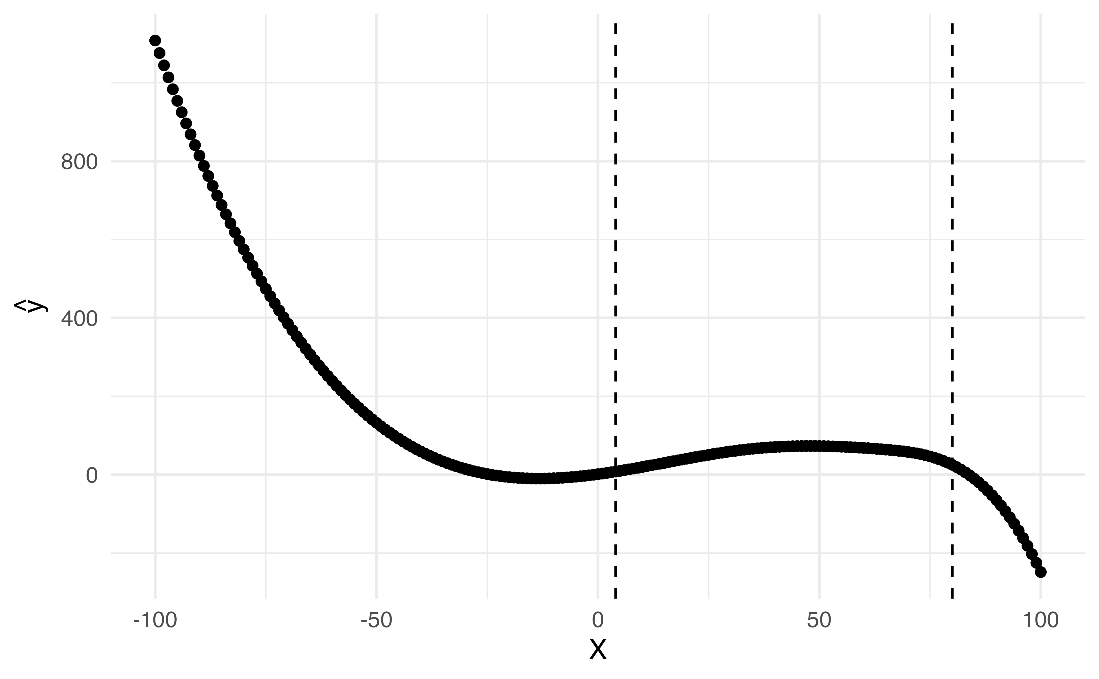
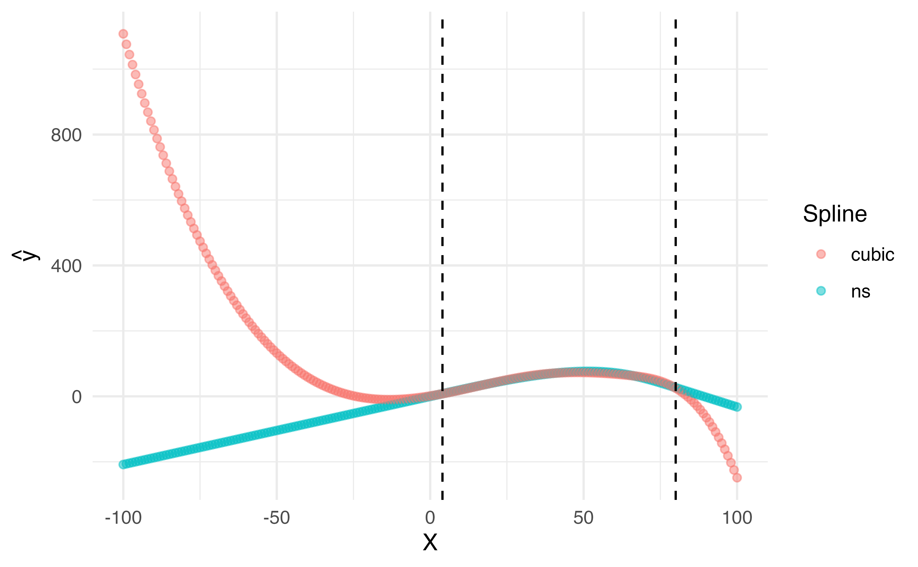
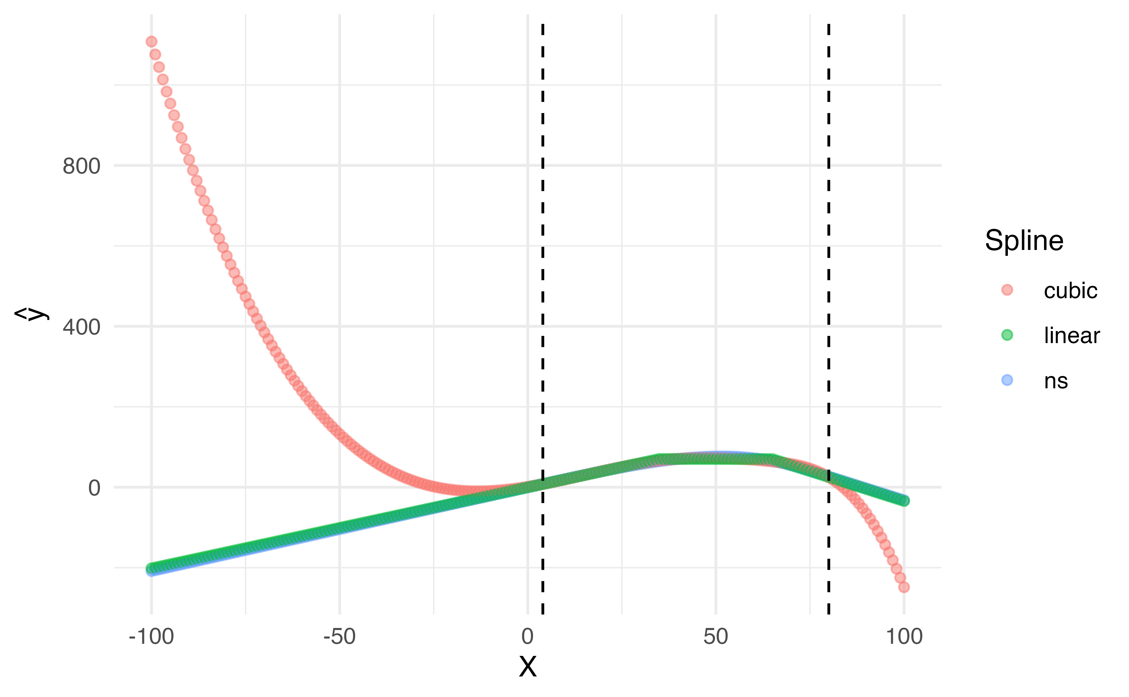
Natural cubic splines
A natural cubic spline extrapolates linearly beyond the boundary knots
This adds 4 extra constraints and allows us to put more internal knots for the same degrees of freedom as a regular cubic spline
Natural Cubic Splines
Natural Cubic Splines
Natural Splines
ggplot (da, aes (x = x, y = value, color = name)) + geom_point (alpha = 0.5 ) + geom_vline (xintercept = c (4 , 80 ), lty = 2 ) + labs (x = "X" ,y = expression (hat (y)),color = "Spline" )
Knot placement
One strategy is to decide \(K\) (the number of knots) in advance and then place them at appropriate quantiles of the observed \(X\)
A cubic spline with \(K\) knots has \(K+3\) parameters (or degrees of freedom!)
A natural spline with \(K\) knots has \(K-1\) degrees of freedom
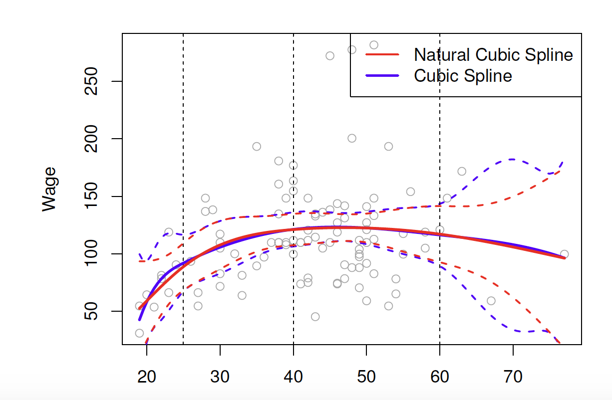
Knot placement
Here is a comparison of a degree-14 polynomial and natural cubic spline (both have 15 degrees of freedom)