02:00
Decision trees - Regression tree building
Lucy D’Agostino McGowan
Decision trees
- Can be applied to regression problems
- Can be applied to classification problems
What is the difference?
Regression trees
Decision tree - Baseball Salary Example
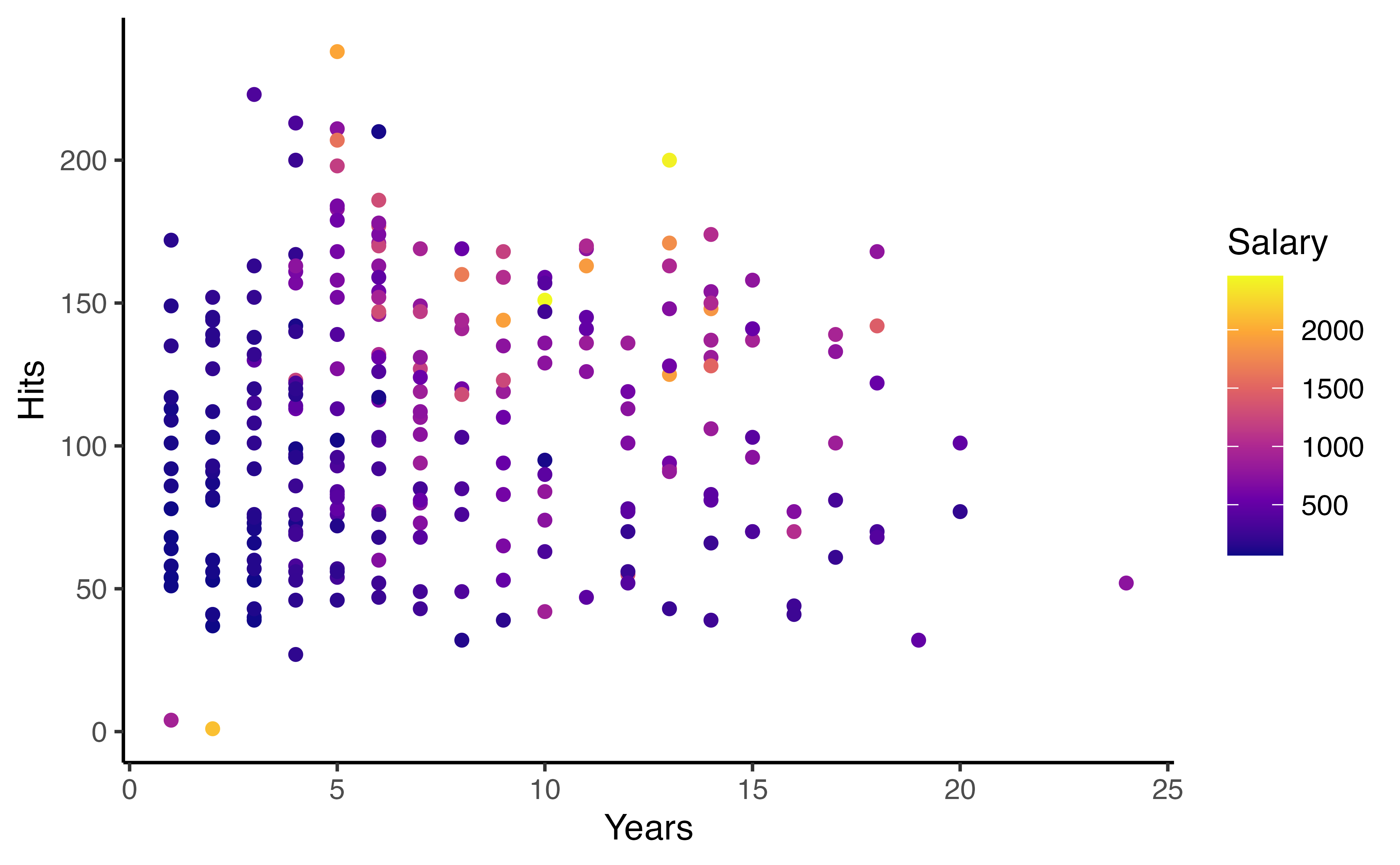
How would you stratify this?
Decision tree - Baseball Salary Example
Let’s walk through the figure
- This is using the
Hittersdata from theISLR📦 - I fit a regression tree predicting the salary of a baseball player from:
- Number of years they played in the major leagues
- Number of hits they made in the previous year
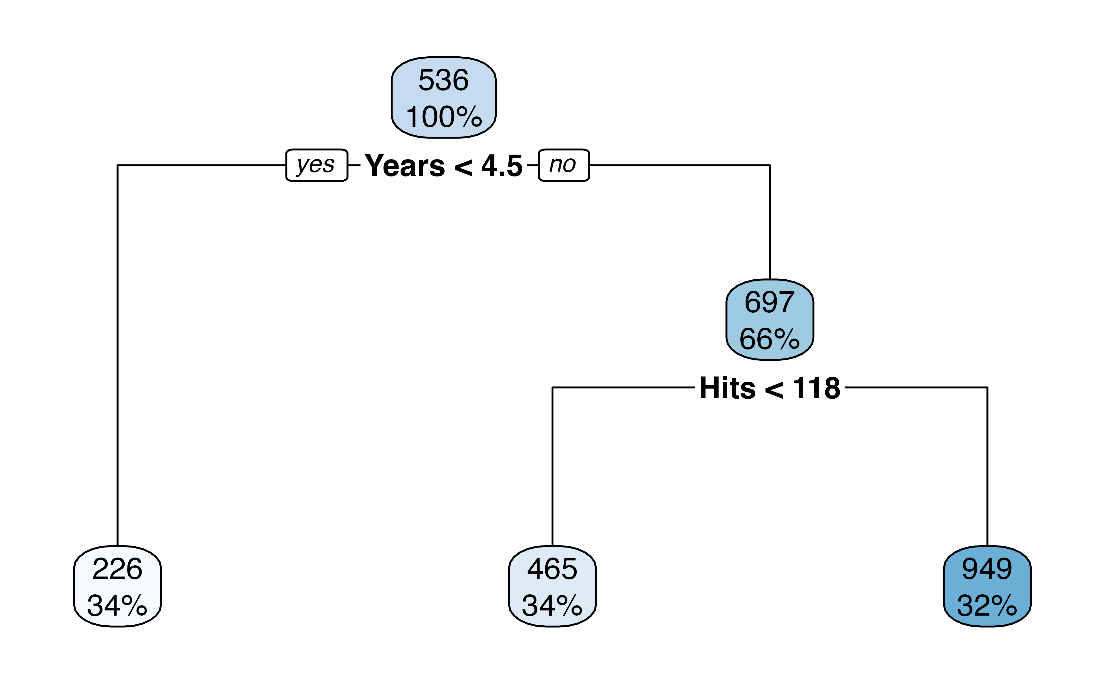
- At each node the label (e.g., \(X_j < t_k\) ) indicates that the left branch that comes from that split. The right branch is the opposite, e.g. \(X_j \geq t_k\).
Let’s walk through the figure
For example, the first internal node indicates that those to the left have less than 4.5 years in the major league, on the right have \(\geq\) 4.5 years.
The number on the top of the nodes indicates the predicted Salary, for example before doing any splitting, the average Salary for the whole dataset is 536 thousand dollars.
This tree has two internal nodes and three termninal nodes
Decision tree - Baseball Salary Example

Decision tree - Baseball Salary Example
Decision tree - Baseball Salary Example
Decision tree - Baseball Salary Example
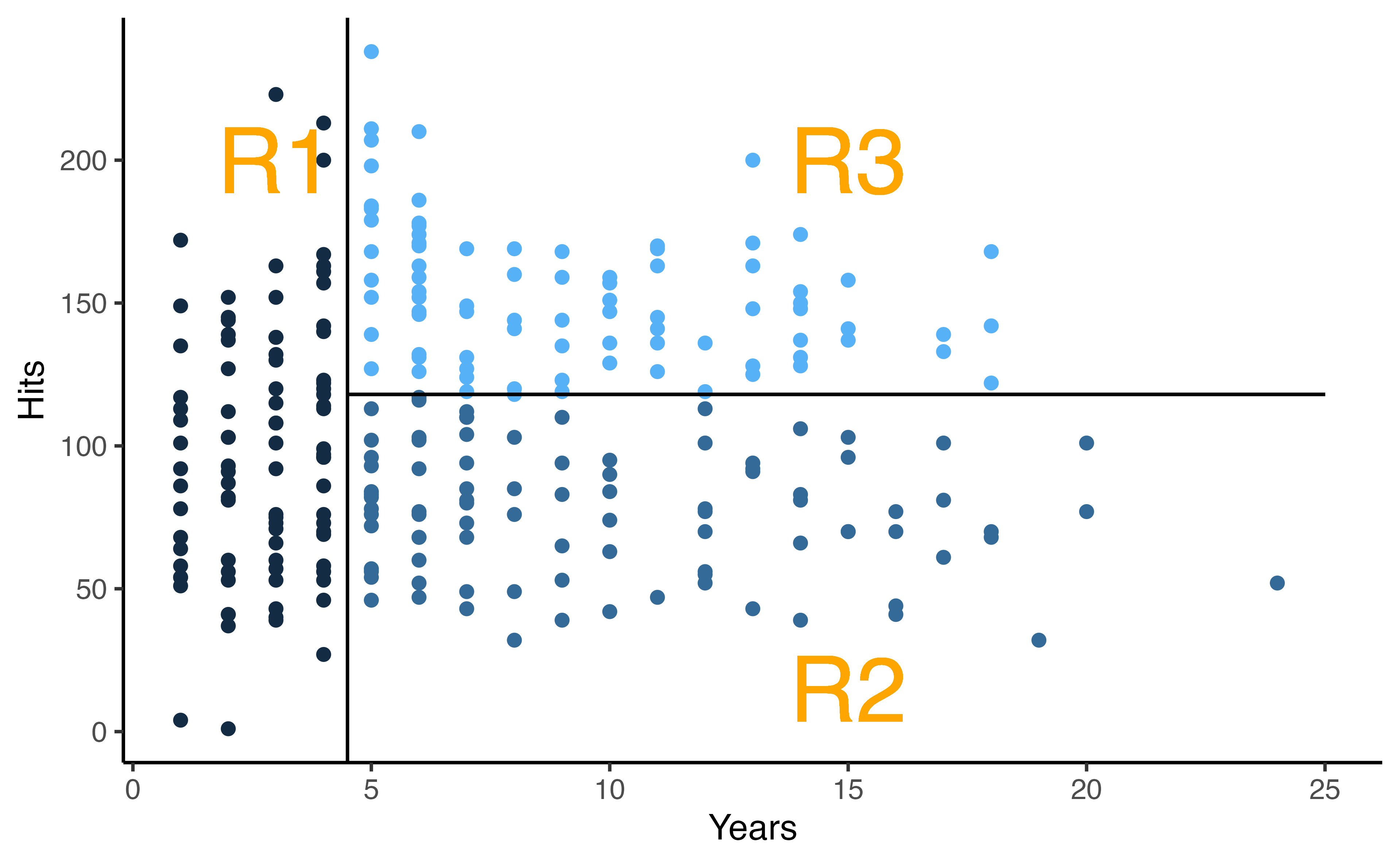
Terminology
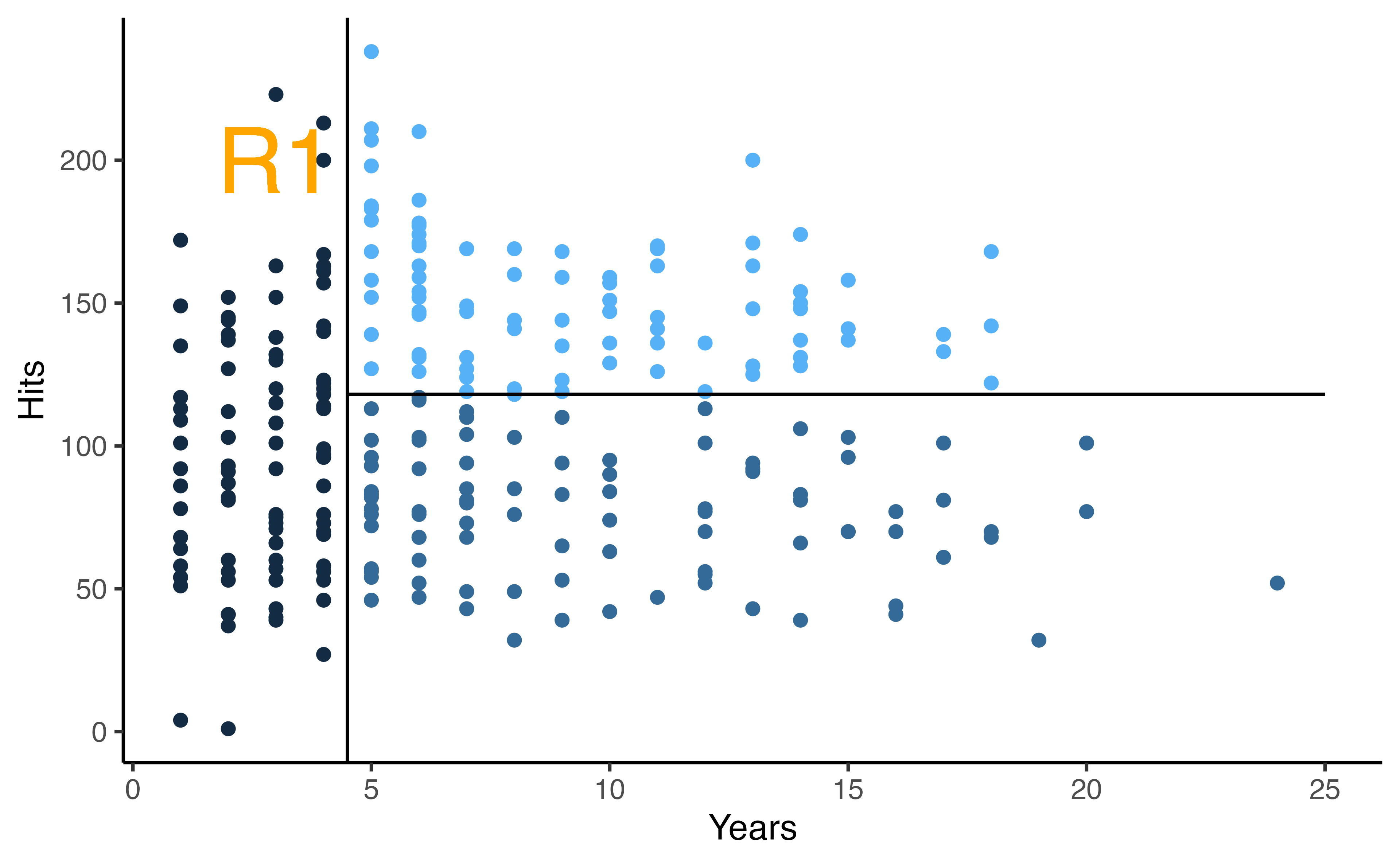
- 🌴 The final regions, \(R_1, R_2, R_3\) are called terminal nodes
- 🌴 You can think of the trees as upside down, the leaves are at the bottom
- 🎋 The splits are called internal nodes
Interpretation of results
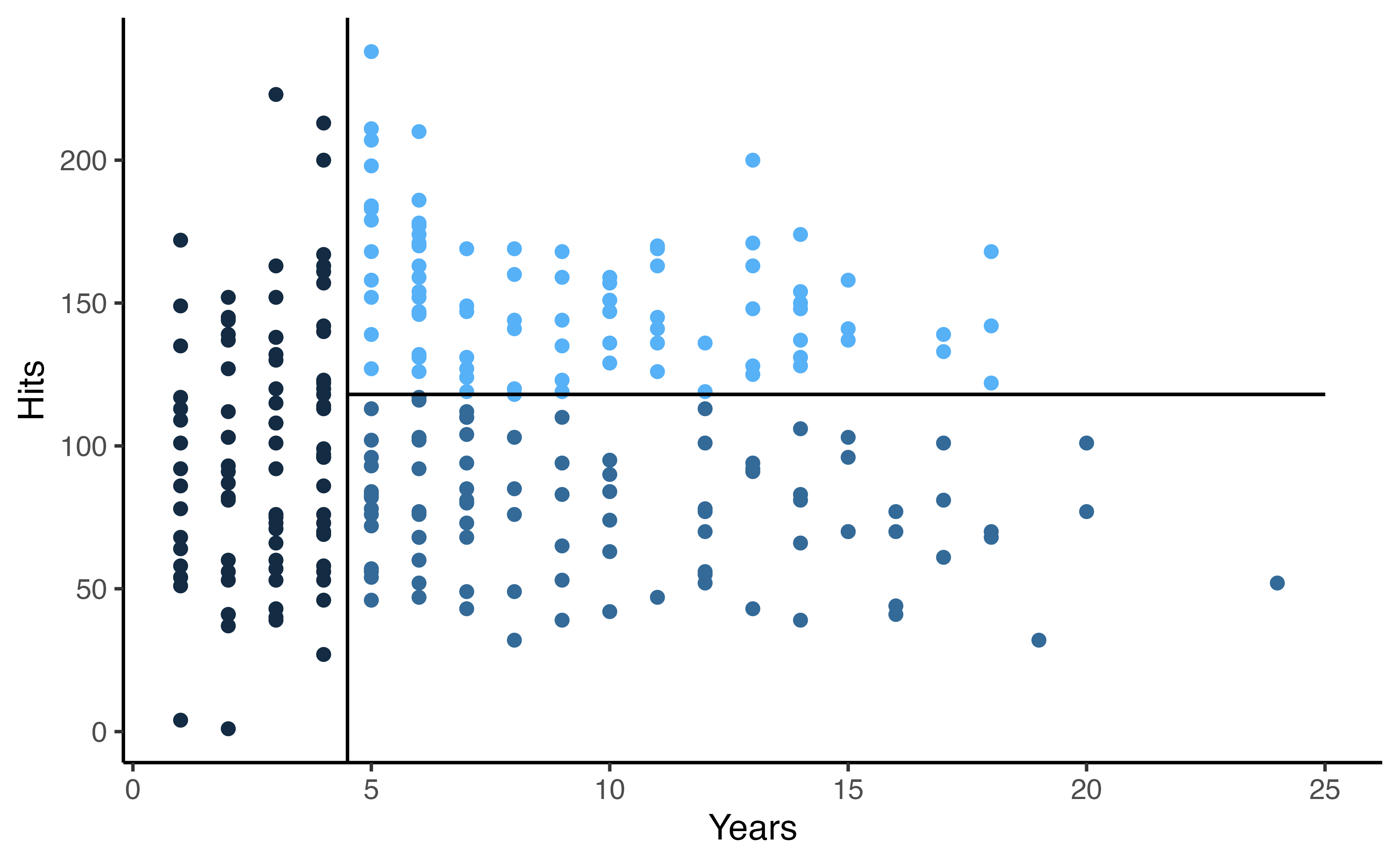
Yearsis the most important factor in determiningSalary; players with less experience earn lower salariesGiven that a player is less experienced, the number of
Hitsseems to play little role in theSalaryAmong players who have been in the major leagues for 4.5 years or more, the number of
Hitsmade in the previous year does affectSalary, players with moreHitstend to have higher salariesThis is probably an oversimplification, but see how easy it is to interpret!
Interpreting decision trees
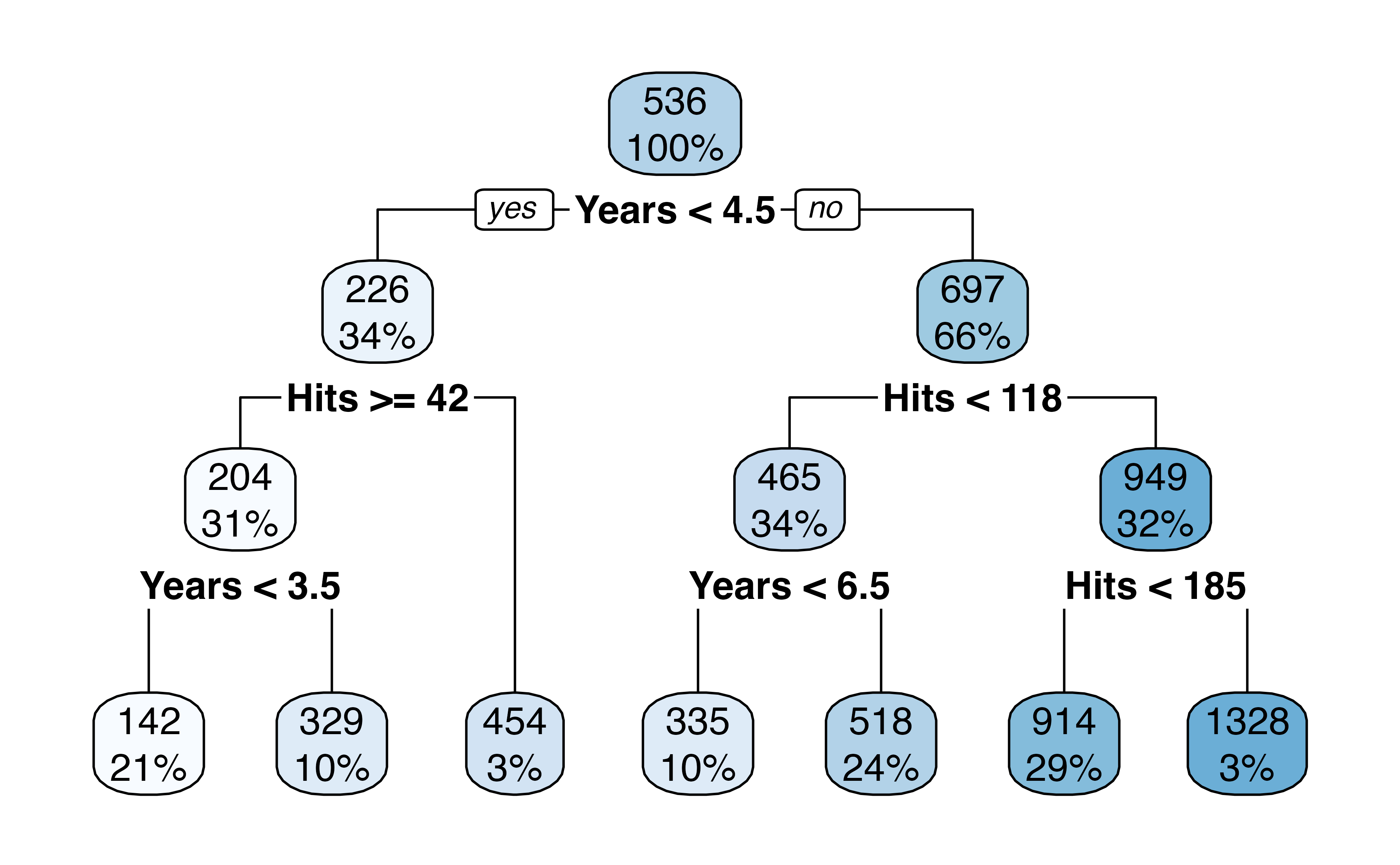
- How many internal nodes does this plot have? How many terminal nodes?
- What is the average Salary for players who have more than 6.5 years in the major leagues but less than 118 Hits? What % of the dataset fall in this category?
The tree building process
- Divide the predictor space (the set of possible values for \(X_1, X_2, \dots, X_p\) ) into \(J\) distinct non-overlapping regions, \(R_1, R_2, \dots R_j\)
- For every observation that falls into the region \(R_j\), we make the same prediction, the mean response value for the training observations in \(R_j\)
The tree building process
The regions could have any shape, but we choose to divide the predictor space into high-dimensional boxes for simplicity and ease of interpretation
The goal is to find boxes, \(R_1, \dots, R_j\) that minimize the RSS, given by
\(\sum_{j=1}^J\sum_{i\in R_j}(y_i-\hat{y}_{R_j})^2\) where \(\hat{y}_{R_j}\) is the mean response for the training observations within the \(j\)th box.
The tree building process
It is often computationally infeasible to consider every possible partition of the feature space into \(J\) boxes
Therefore, we take a top-down, greedy approach known as recursive binary splitting
This is top-down because it begins at the top of the tree and then splits the predictor space successively into two branches at a time
It is greedy because at each step the best split is made at that step (instead of looking forward and picking a split that may result in a better tree in a future step)
The tree building process
First select the predictor \(X_j\) and the cutpoint \(s\) such that splitting the predictor space into \(\{X|X_j < s\}\) and \(\{X|X_k\geq s\}\) leads to the greatest possible reduction in RSS
We repeat this process, looking for the best predictor and cutpoint to split the data within each of the resulting regions
Now instead of splitting the entire predictor space, we split one of the two previously identified regions, now we have three regions
The tree building process
- Then we look to split one of these three regions to minimize the RSS
- This process continues until some stopping criteria are met. 🛑 e.g., we could stop when we have created a fixed number of regions, or we could keep going until no region contains more than 5 observations, etc.
Draw a partition
Draw an example of a partition of a two-dimensional feature space that could result from recursive binary splitting with six regions. Label your figure with the regions, \(R_1, \dots, R_6\) as well as the cutpoints \(t_1, t_2, \dots\). Draw a decision tree corresponding to this partition.
05:00
Decision tree predictions
- Predict the response for a test observation using the mean of the training observations in the region that the test observation belongs to
What could potentially go wrong with what we have described so far?
- The process may produce good predictions on the training set but is likely to overfit!
Pruning a tree
Do you love the tree puns? I DO!
A smaller tree (with fewer splits, that is fewer regions \(R_1,\dots, R_j\) ) may lead to lower variance and better interpretation at the cost of a little bias
A good strategy is to grow a very large tree, \(T_0\), and then prune it back to obtain a subtree
For this, we use cost complexity pruning (also known as weakest link 🔗 pruning)
Consider a sequence of trees indexed by a nonnegative tuning parameter, \(\alpha\). For each \(\alpha\) there is a subtree \(T \subset T_0\) such that \(\sum_{m=1}^{|T|}\sum_{i:x_i\in R_m}(y_i-\hat{y}_{R_m})^2+\alpha|T|\) is as small as possible.
Pruning
\[\sum_{m=1}^{|T|}\sum_{i:x_i\in R_m}(y_i-\hat{y}_{R_m})^2+\alpha|T|\]
\(|T|\) indicates the number of terminal nodes of the tree \(T\)
\(R_m\) is the box (the subset of the predictor space) corresponding to the \(m\)th terminal node
\(\hat{y}_{R_m}\) is the mean of the training observations in \(R_m\)
Choosing the best subtree
The tuning parameter, \(\alpha\), controls the trade-off between the subtree’s complexity and its fit to the training data
How do you think you could select \(\alpha\)?
You can select an optimal value, \(\hat{\alpha}\) using cross-validation!
Then return to the full dataset and obtain the subtree using \(\hat{\alpha}\)
Summary regression tree algorithm
Use recursive binary splitting to grow a large tree on the training data, stop when you reach some stopping criteria
Apply cost complexity pruning to the larger tree to obtain a sequence of best subtrees, as a function of \(\alpha\)
Use K-fold cross-validation to choose \(\alpha\). Pick \(\alpha\) to minimize the average error
Return the subtree that corresponds to the chosen \(\alpha\)
The baseball example
1. Randomly divide the data in half, 132 training observations, 131 testing
2. Create cross-validation object for 6-fold cross validation
3. Create a model specification that tunes based on complexity, \(\alpha\) and add to workflow
What is my tree depth for my “large” tree?
4. Fit the model on the cross validation set
What \(\alpha\)s am I trying?
5. Choose \(\alpha\) that minimizes the RMSE
# A tibble: 5 × 7
  cost_complexity .metric .estimator  mean     n std_err .config
            <dbl> <chr>   <chr>      <dbl> <int>   <dbl> <chr>
1            0.01 rmse    standard    422.     6    33.6 Preprocessor1_Model1
2            0.02 rmse    standard    423.     6    32.0 Preprocessor1_Model2
3            0.03 rmse    standard    425.     6    31.9 Preprocessor1_Model3
4            0.04 rmse    standard    429.     6    32.5 Preprocessor1_Model4
5            0.05 rmse    standard    441.     6    25.3 Preprocessor1_Model5
5. Choose \(\alpha\) that minimizes the RMSE
5. Choose \(\alpha\) that minimizes the RMSE
6. Fit the final model
Final tree
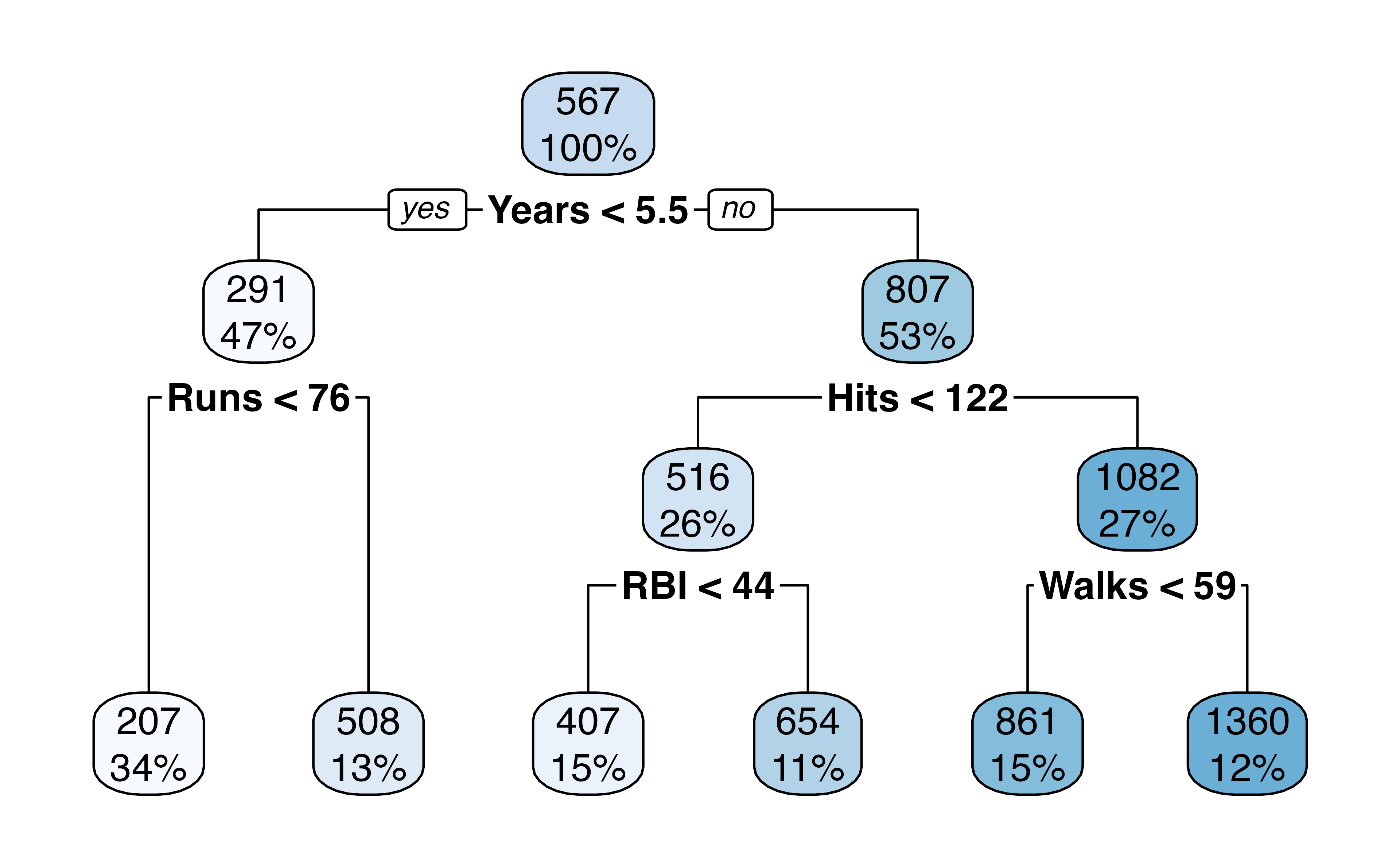
How many terminal nodes does this tree have?
Calculate RMSE on the test data
Application Exercise
Pull in the application exercise files from:
Using the College data from the ISLR package, predict the number of applications received from a subset of the variables of your choice using a decision tree. (Not sure about the variables? Run ?College in the console after loading the ISLR package)
10:00
Dr. Lucy D’Agostino McGowan adapted from slides by Hastie & Tibshirani