Decision trees - Classification trees

Lucy D’Agostino McGowan

Classification Trees

• Very similar to regression trees except it is used to predict a qualitative response rather than a quantitative one

• We predict that each observation belongs to the most commonly occuring class of the training observations in a given region

Fitting classification trees

• We use recursive binary splitting to grow the tree

• Instead of RSS, we can use:

• Gini index: \(G = \sum_{k=1}^K \hat{p}_{mk}(1-\hat{p}_{mk})\)

• This is a measure of total variance across the \(K\) classes. If all of the \(\hat{p}_{mk}\) values are close to zero or one, this will be small

• The Gini index is a measure of node purity small values indicate that node contains predominantly observations from a single class

• In R, this can be estimated using the gain_capture() function.

Classification tree - Heart Disease Example

• Classifying whether 303 patients have heart disease based on 13 predictors (Age, Sex, Chol, etc)

1. Split the data into a cross-validation set

heart_cv <- vfold_cv(heart, v = 5)

How many folds do I have?

2. Create a model specification that tunes based on complexity, \(\alpha\)

tree_spec <- decision_tree(
  cost_complexity = tune(), 
  tree_depth = 10,
  mode = "classification") %>% 
  set_engine("rpart")

wf <- workflow() |>
  add_recipe(
    recipe(HD ~ Age + Sex + ChestPain + RestBP + Chol + Fbs + 
                     RestECG + MaxHR + ExAng + Oldpeak + Slope + Ca,
    data = heart
    )
  ) |>
  add_model(tree_spec)

3. Fit the model on the cross validation set

grid <- expand_grid(cost_complexity = seq(0.01, 0.05, by = 0.01))
model <- tune_grid(wf,
                   grid = grid,
                   resamples = heart_cv,
                   metrics = metric_set(gain_capture, accuracy)) 

What \(\alpha\)s am I trying?

5. Choose \(\alpha\) that minimizes the Gini Index

best <- model %>%
  select_best(metric = "gain_capture")

6. Fit the final model

final_wf <- wf |>
  finalize_workflow(best)

final_model <- fit(final_wf, data = heart)

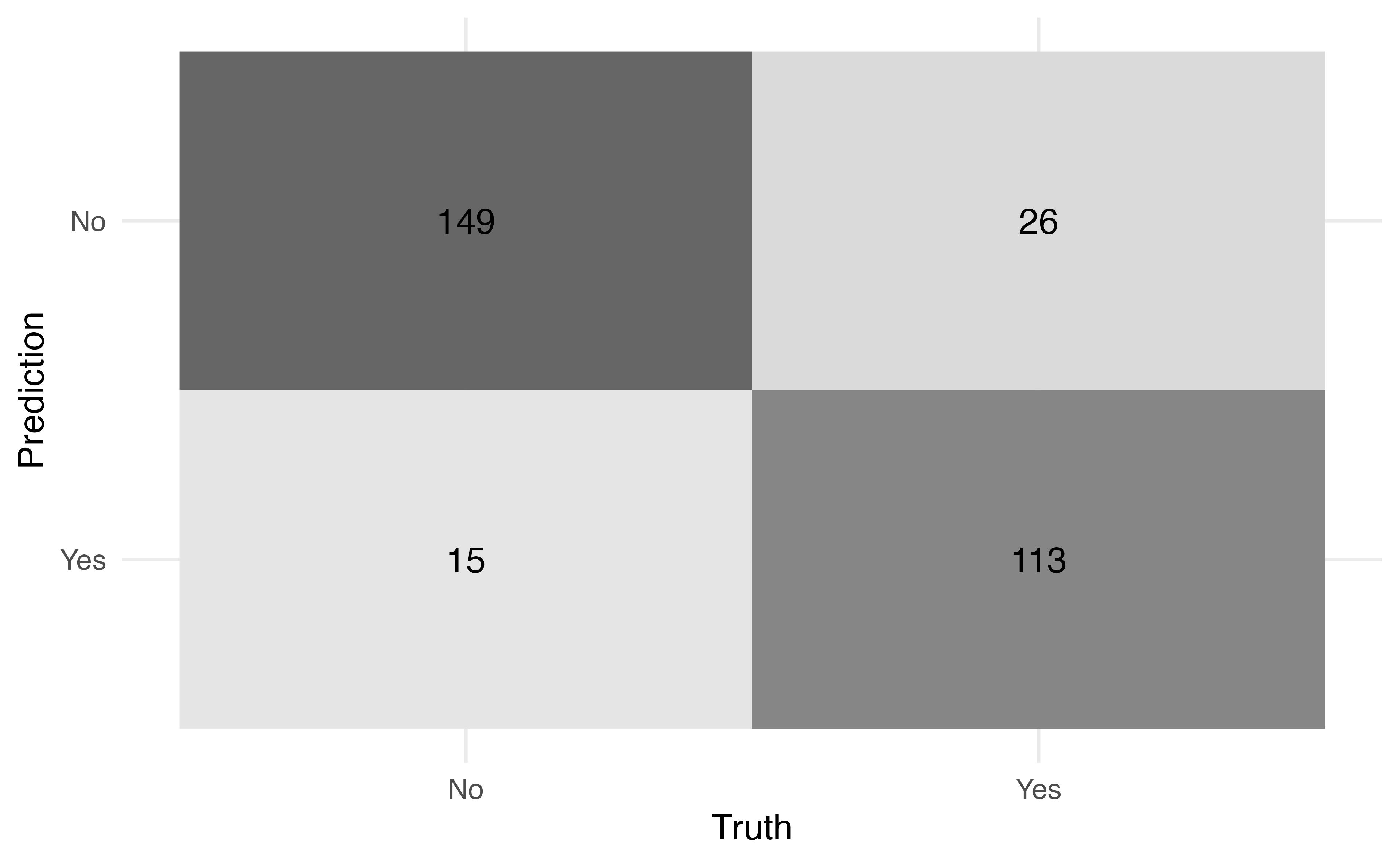
7. Examine how the final model does on the full sample

final_model %>%
  predict(new_data = heart) %>%
  bind_cols(heart) %>%
  conf_mat(truth = HD, estimate = .pred_class) %>%
  autoplot(type = "heatmap")

Decision trees

Pros

• simple
• easy to interpret

Cons

• not often competitive in terms of predictive accuracy
• Next we will discuss how to combine multiple trees to improve accuracy