Random Forests

Lucy D’Agostino McGowan

Random forests

Do you ❤️ all of the tree puns?

• Random forests provide an improvement over bagged trees by way of a small tweak that decorrelates the trees

• By decorrelating the trees, this reduces the variance even more when we average the trees!

Random Forest process

• Like bagging, build a number of decision trees on bootstrapped training samples

• Each time the tree is split, instead of considering all predictors (like bagging), a random selection of \(m\) predictors is chosen as split candidates from the full set of \(p\) predictors

• The split is allowed to use only one of those \(m\) predictors

• A fresh selection of \(m\) predictors is taken at each split

• typically we choose \(m \approx \sqrt{p}\)

Choosing m for Random Forest

Let’s say you have a dataset with 100 observations and 9 variables, if you were fitting a random forest, what would a good \(m\) be?

01:00

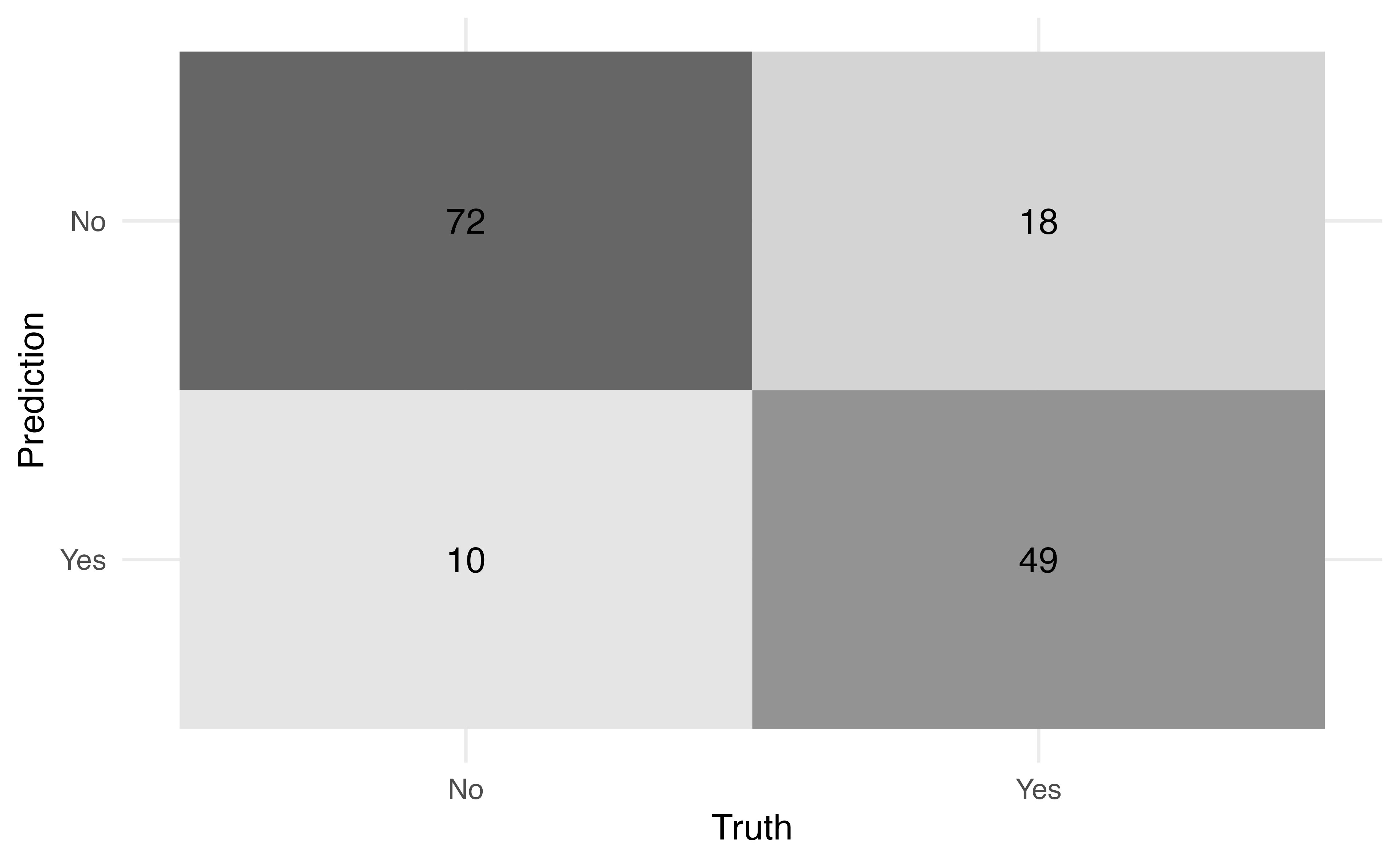
The heart disease example

Recall that we are predicting whether a patient has heart disease from 13 predictors

1. Randomly divide the data in half, 149 training observations, 148 testing

set.seed(77)
heart_split <- initial_split(heart, prop = 0.5)
heart_train <- training(heart_split)

2. Create model specification

model_spec <- rand_forest(
  mode = "classification",
  mtry = ---
) |> 
  set_engine("ranger")

mtry here is m. If we are doing bagging what do you think we set this to?

2. Create bagging specification

bagging_spec <- rand_forest(
  mode = "classification",
  mtry = 13 #<<
) |> 
  set_engine("ranger")

What would we change mtry to if we are doing a random forest?

2. Create Random Forest specification

rf_spec <- rand_forest(
  mode = "classification",
  mtry = 3 #<<
) |> 
  set_engine("ranger")

• The default for rand_forest is floor(sqrt(# predictors)) (so 3 in this case)

3. Create the workflow

wf <- workflow() |>
  add_recipe(
    recipe(
      HD ~ Age + Sex + ChestPain + RestBP + Chol + Fbs + 
               RestECG + MaxHR + ExAng + Oldpeak + Slope + Ca + Thal,
             data = heart_train
    )
  ) |>
  add_model(rf_spec)

4. Fit the model

model <- fit(wf, data = heart_train)

5. Examine how it looks in the test data

heart_test <- testing(heart_split)
model |>
  predict(new_data = heart_test) |>
  bind_cols(heart_test) |>
  conf_mat(truth = HD, estimate = .pred_class) |>
  autoplot(type = "heatmap")

Application Exercise

• Open your last application exercise
• Refit your model as a random forest

10:00