Neural Networks
Neural Network
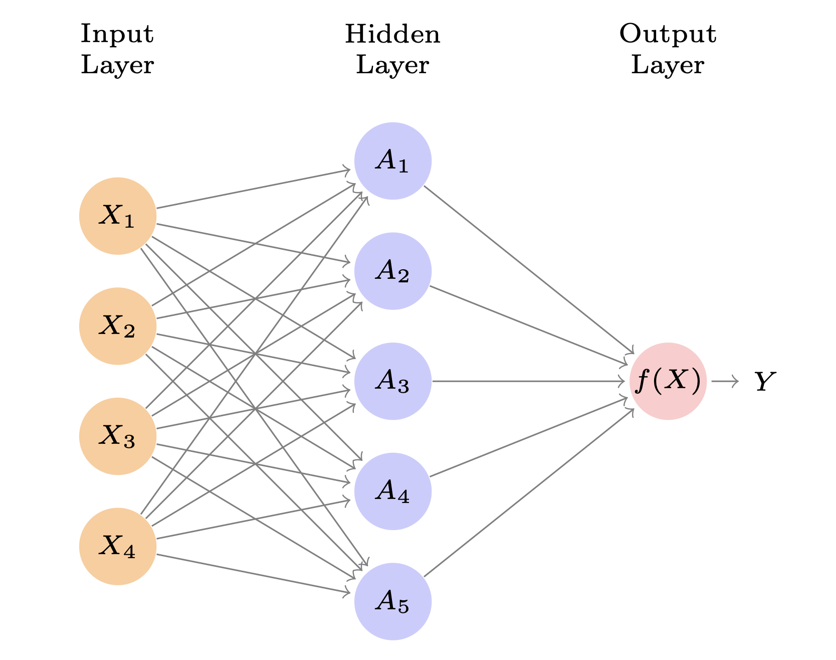
\[ f(X) = \beta_0 + \sum_{k=1}^K\beta_kh_k(X)\\ =\beta_0 + \sum_{k=1}^K\beta_kg(w_{k0}+\sum_{j=1}^p w_{kj}X_j) \]
Neural Network
Neural Network
- \(A_k = h_k(X) = g(w_{k0} + \sum_{j=1}^pw_{kj}X_j)\)
- These are called the activations in the hidden layer
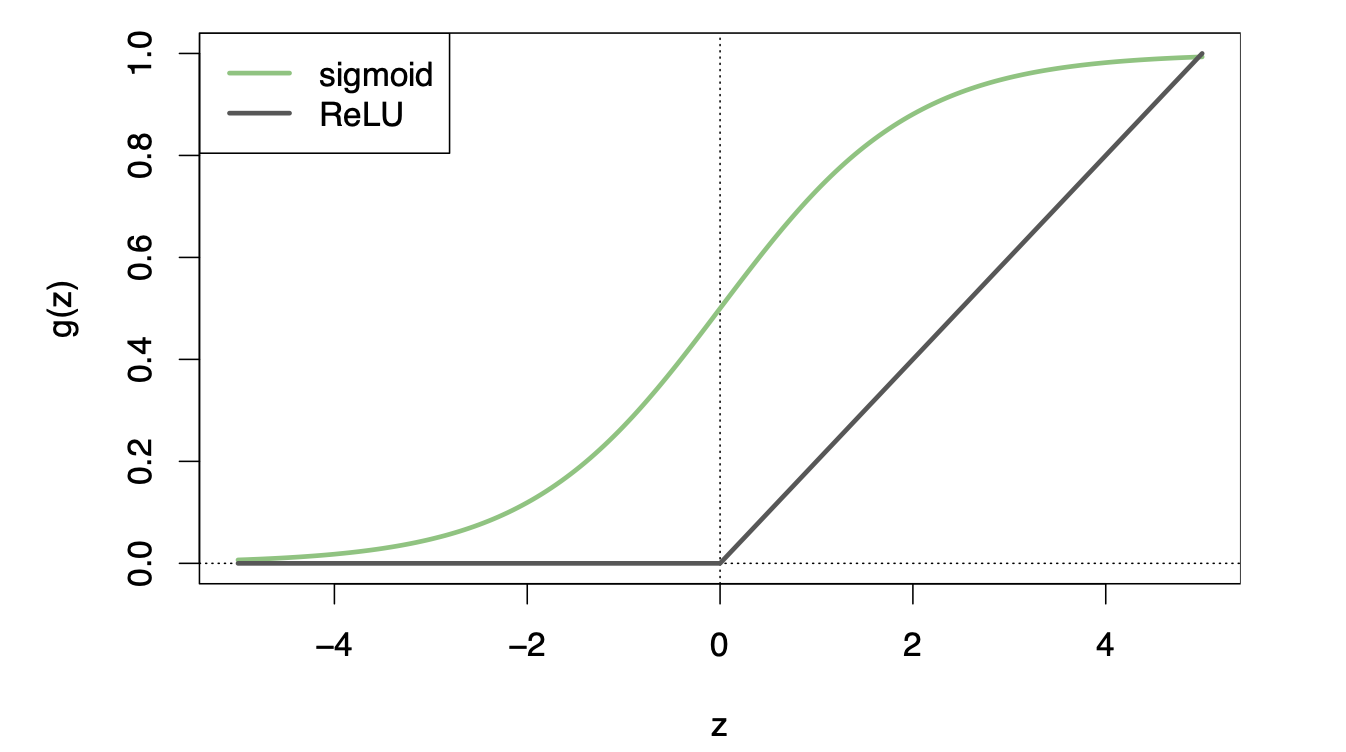
- \(g(z)\) is called the activation function
- Popular \(g(z)\) functions are the sigmoid and rectified linear
Neural Network
Neural Network
- Activation functions are usually nonlinear otherwise the model just collapses to a linear model
- The activations (\(A_k\)) are nonlinear transformations of linear combinations of the features (the features are the input predictors, \(X\))
- We can have multiple “hidden layers”
- The model is fit by minimizing RSS!
- It is fit in a slow (using a learning rate, like we did for boosting), in an iterative fashion using gradient descent, you can prevent overfitting
Gradient Descent
Gradient descent is an optimization algorithm used to minimize a function by iteratively moving in the direction of steepest descent as defined by the negative of the gradient.
Here is a simple example of gradient descent: we have a feature \(x\) and an outcome \(y\) and want to find the line that best fits the data
The “loss function” can be mean squared error \(L = \frac{1}{n}\sum_{i=1}^{n}(y_i - (\hat\beta_0 + \hat\beta_1x_i ))^2\)
Gradient Descent
We can use gradient descent to find the values of \(\hat\beta_0\) and \(\hat\beta_1\) that minimize the MSE.
The gradient of the loss function with respect to the parameters \(\beta_0\) is: \(\frac{\partial L}{\partial \beta_0} = \frac{-2}{n}\sum_{i=1}^{n}(y_i - (\beta_0 + \beta_1x_i))\)
And for \(\beta_1\): \(\frac{\partial L}{\partial \beta_1} = \frac{-2}{n}\sum_{i=1}^{n}x_i(y_i - (\beta_0 + \beta_1x_i))\)
We can then update the values of \(\hat\beta_0\) and \(\hat\beta_1\) using the following equations: \(\beta_{i,new} = \beta_i - \alpha \frac{\partial L}{\partial \beta_i}\) where \(\alpha\) is the learning rate.
Gradient Descent
Here’s an example of gradient descent with a small dataset:
| x | y |
|---|---|
| 1 | 1 |
| 2 | 3 |
| 3 | 5 |
| 4 | 7 |
Gradient Descent
Keras
- Keras is an open-source neural network library written in Python.
- It is designed to provide a high-level API for building and training deep learning models.
- It is built on top of other popular deep learning libraries, such as TensorFlow
- We are going to run Keras from R using Python behind the scenes
Application Exercise
- Pull in the application exercise files from:
- Run
install.packages("keras")once in the console - Run
keras::install_keras()once in the console - When it asks if you want to install Miniconda type
Y
02:00
Example: Hitters Data
- We are trying to predict the Salary for baseball players
- We have 19 predictors
- We will use a single layer neural network 🎉
Application Exercise
- Create a recipe that uses all of the included variables to predict Salary
- Remove any missing data for the outcome, impute data for the remaining predictors (HINT: in
step_naomit()setskip = FALSEto make sure it does this when we are prepping the data) - Make all nominal variables dummy variables
- Normalize all predictors using
step_normalize()
05:00
Example: Hitters Data
Example: Hitters Data
rec <- recipe(Salary ~ ., data = Hitters) |>
  step_naomit(Salary, skip = FALSE) |>
  step_impute_knn(all_predictors()) |>
  step_dummy(all_nominal_predictors()) |>
  step_normalize(all_predictors())

set.seed(1)
splits <- initial_split(Hitters, prop = 2/3)
train <- training(splits)
test <- testing(splits)

training_processed <- prep(rec) |> bake(new_data = train)
testing_processed <- prep(rec) |> bake(new_data = test)

training_matrix_x <- training_processed |> select(-Salary) |> as.matrix()
testing_matrix_x <- testing_processed |> select(-Salary) |> as.matrix()
Application Exercise
- Using the Hitters data, split into 2/3 training and 1/3 testing data
- Create datasets for the training and testing data
- Run the recipe on the training and testing data
- Extract just the predictors into a data frame and then convert this into a matrix for both the training and testing pre-processed data
04:00
Example: Hitters Data
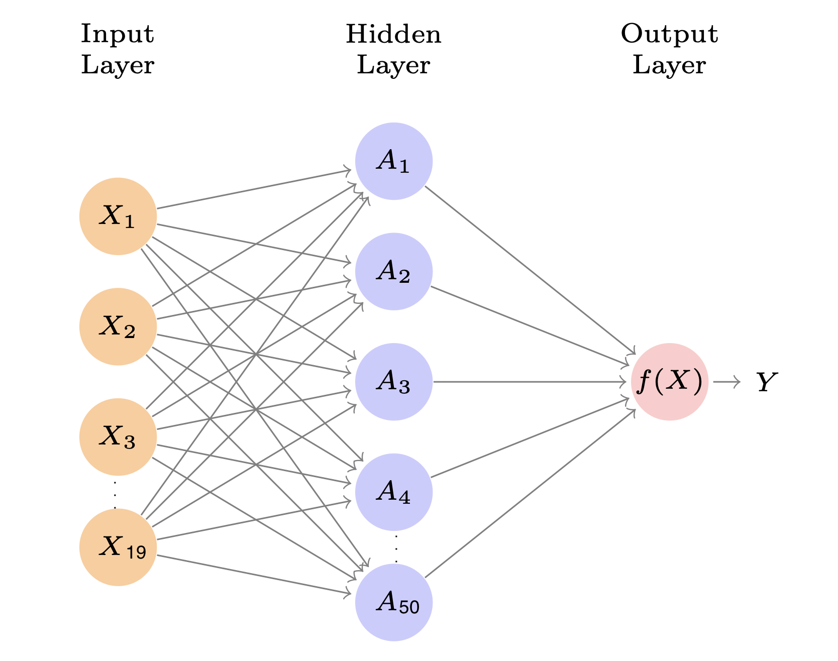
- Let’s fit a model with 50 activations in a hidden layer using a rectified linear (ReLU) activation function
- Since we have 19 variables, this first layer has \((19+1)\times 50\) parameters
- Then we will have an output with just one unit and no activation function, since we just want a single number quantitative output (this results in \((50 + 1)\times 1\) parameters)
- Overall, this model has 1,051 parameters 😱
Example:: Hitters Data
Example: Hitters Data
- Overall, this model has 1,051 parameters 😱
- Let’s add in a “dropout layer” – this means a specified percent of the 50 activations from the previous layer will be set to 0 in each iteration of stochastic gradient descent algorithm
- We can specify a batch size such that at each step of the stochastic gradient descent a random selection of training observations will be used to compute the gradient. Let’s do 32 (meaning each iteration will have 32/176 = 5.5 SGD steps)
- We can also set how long we want the model to run (how many epochs or iterations) Let’s do 100
Example: Hitters Data
mod <- keras_model_sequential() |>
  layer_dense(units = 50, activation= "relu", input_shape = 19) |>
  layer_dropout(rate = 0.4) |>
  layer_dense(units = 1) |>
  compile(loss = "mse",
           metrics = list("mse")) |>
  fit(training_matrix_x,
      training_processed$Salary,
      epochs = 100,
      batch_size = 32,
      validation_data = list(testing_matrix_x, testing_processed$Salary))
Example: Hitters Data
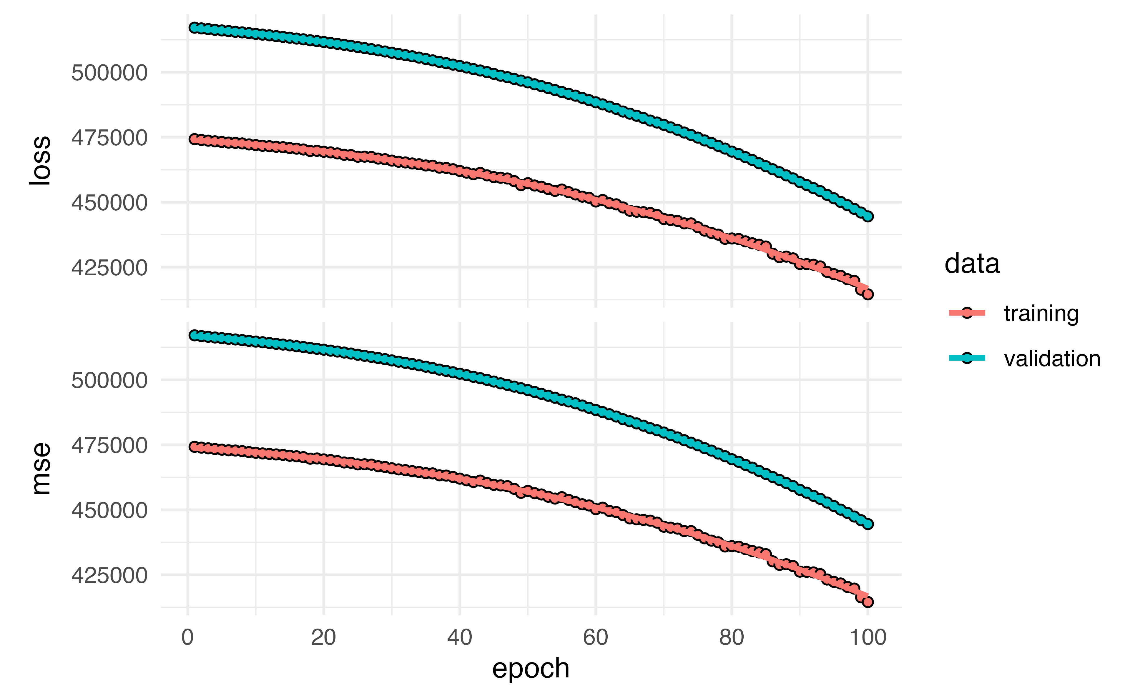
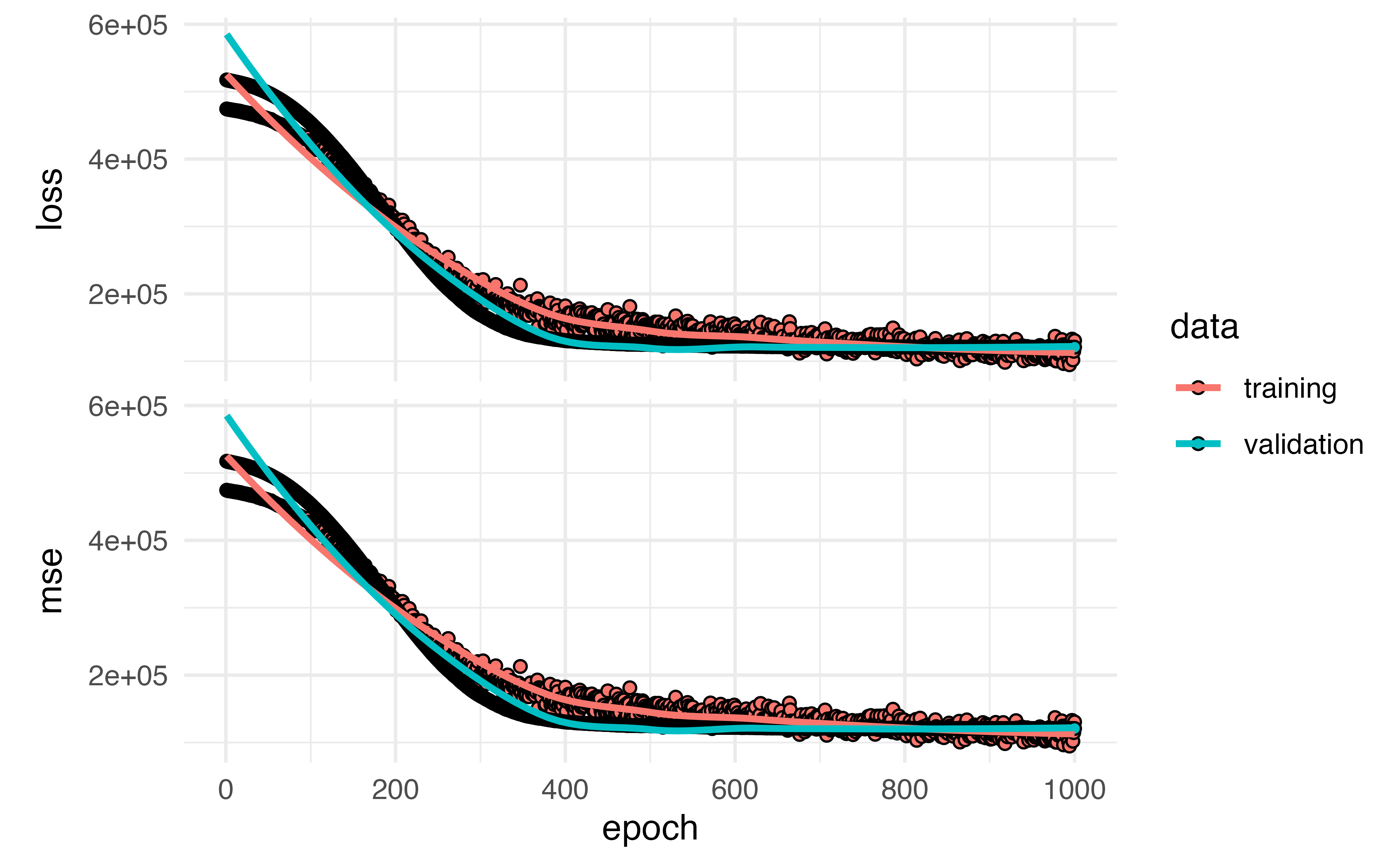
Application Exercise
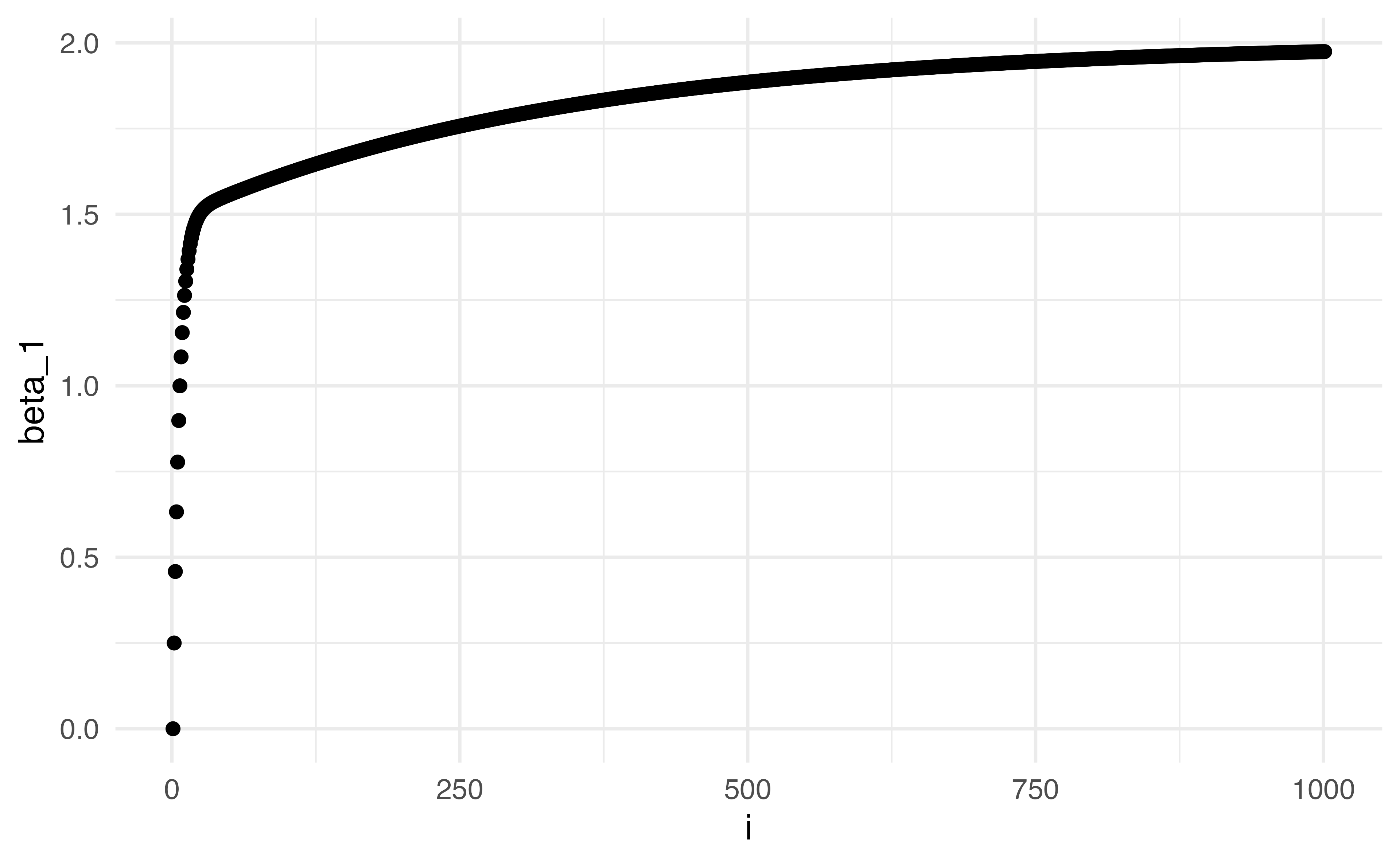
- Fit a model with 40 activations in a hidden layer with 50% dropout and a batch size of 30
- Run your model for 1,000 iterations (epochs)
- Use your testing data as validation
- Plot the output
06:00
Example:: Hitters Data
mod <- keras_model_sequential() |>
  layer_dense(units = 40, activation= "relu", input_shape = 19) |>
  layer_dropout(rate = 0.5) |>
  layer_dense(units = 1) |>
  compile(loss = "mse",
           metrics = list("mse")) |>
  fit(training_matrix_x,
      training_processed$Salary,
      epochs = 1000,
      batch_size = 30,
      validation_data = list(testing_matrix_x, testing_processed$Salary))
Example: Hitters Data
Example: Classifying numbers
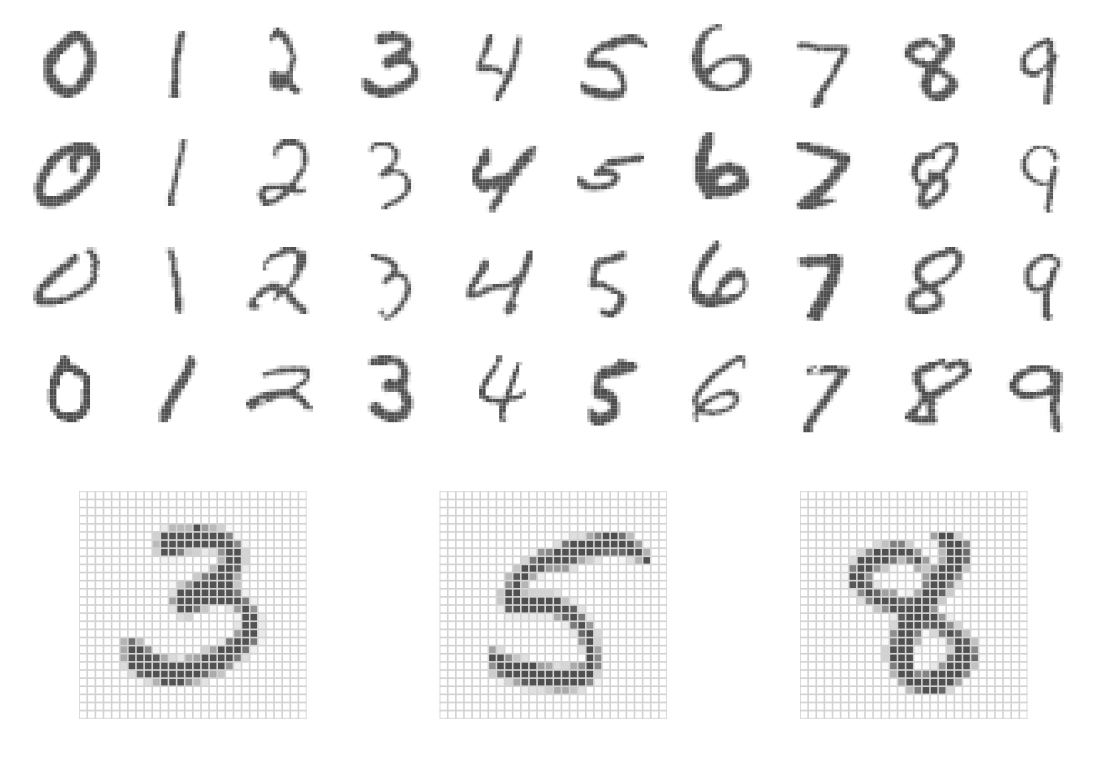
- Handwritten digits 28x28 grayscale images
- features: 28x28 = 784 pixel grayscale values from 0 to 255
- outcome: labels 0-9
- We want to build a prediction model to predict the written number
Example: Classifying numbers
- Let’s build a two layer neural network with 256 units in the first layer, 128 units in the second, and 10 units at the output layer (for the digits 0-9)
- The first layer will have \((784 + 1) \times 256\) parameters (Why?)
- The second layer will have \((256 + 1)\times 128\) parameters
- The output layer will have \((128 + 1) \times 10\) parameters
Example: Classifying numbers
How many parameters does this model have in total?
- \((784 + 1) \times 256 + (256 + 1) \times 128 + (128 + 1)\times 10=235,146\)
- Why are there +1? Those are for the intercepts (for some reason, the machine learning folks call these biases)
- The “parameters” are referred to as weights
Example: Classifying numbers
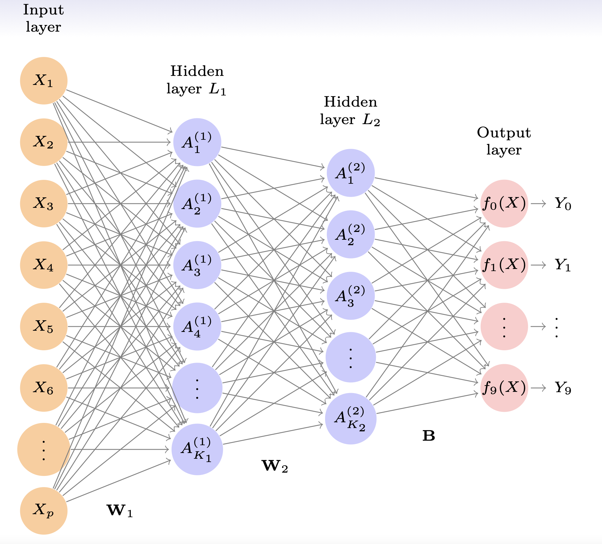
Output layer details
- So far, we have just been talking about linear combinations (which sounds like regression), but we want to turn these into categorical predictions (i.e. the probability that the input is in each of the categories)
- The output layer starts with 10 linear combinations of the activations from the second layer: \(Z_m = \beta_{m0} + \sum_{l=1}^{K_2}\beta_{ml}A_{l}^{(2)}, m = 0, 1, \dots, 9\)
- Then the output activation function encodes the softmax function like this: \(f_m(X) = P(Y = m | X) = \frac{e^{Z_m}}{\sum_{l=0}^9 e^{Z_l}}\)
Example: Classifying numbers
- Since this is a classification problem, we need to pick something to minimize
- We can minimize the negative multinomial log-likelihood (cross-entropy)
\[ -\sum_{i=1}^n\sum_{m=0}^9 y_{im}log(f_m(x_i)) \]
R code
model <- keras_model_sequential() |>
  layer_dense(units = 256, activation = "relu", input_shape = 784) |>
  layer_dropout(rate = 0.4) |>
  layer_dense(units = 128, activation = "relu") |>
  layer_dropout(rate = 0.3) |>
  layer_dense(units = 10, activation = "softmax")

summary(model)
Model: "sequential"
________________________________________________________________________________
Layer (type) Output Shape Param #
================================================================================
dense_2 (Dense) (None, 256) 200960
dropout_1 (Dropout) (None, 256) 0
dense_1 (Dense) (None, 128) 32896
dropout (Dropout) (None, 128) 0
dense (Dense) (None, 10) 1290
================================================================================
Total params: 235,146
Trainable params: 235,146
Non-trainable params: 0
________________________________________________________________________________R Code
R code
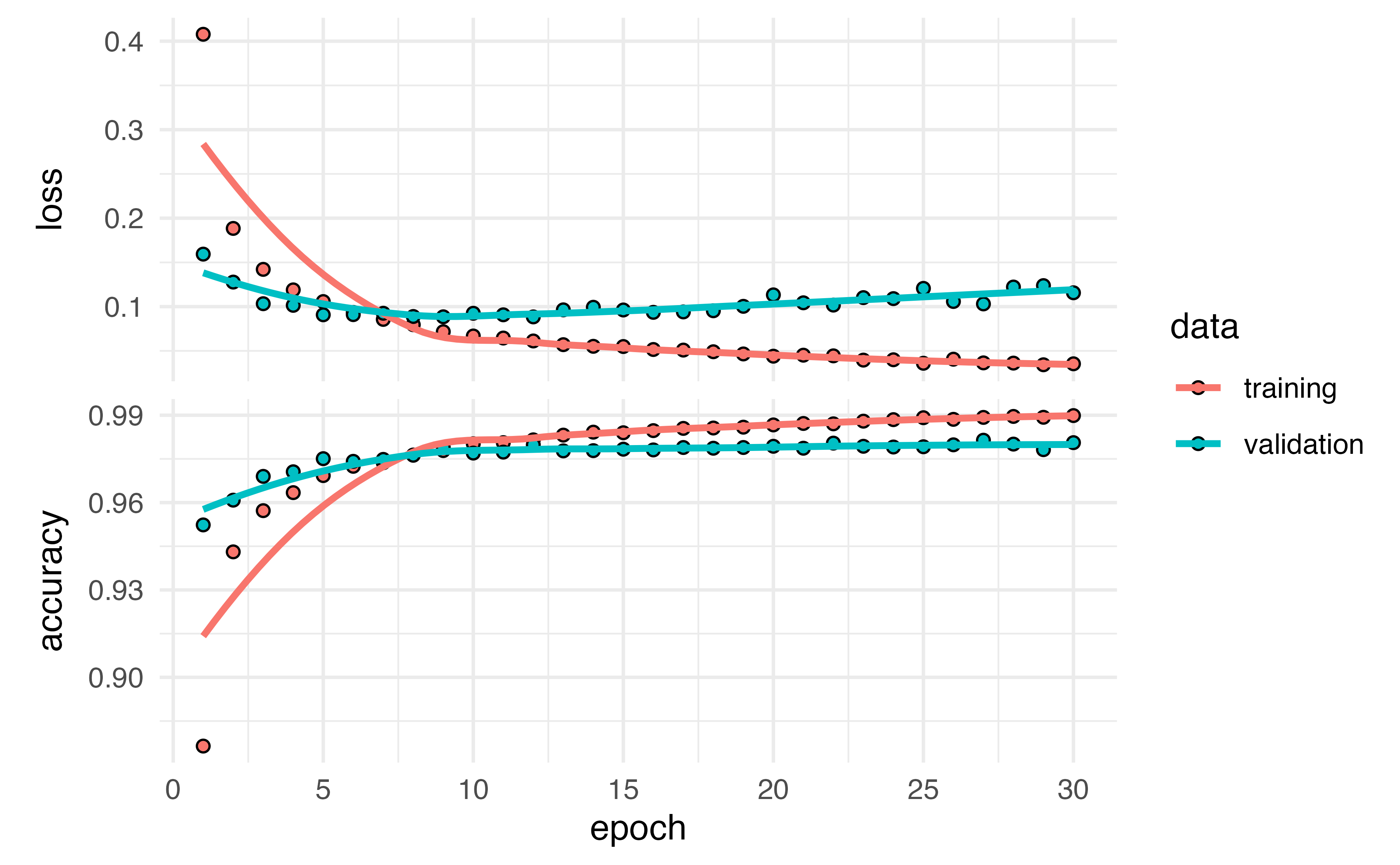
Accuracy
GPT
- GPT stands for Generative Pre-trained Transformer.
- Generative model trained to generate human-like text.
- Pre-trained on massive amounts of text data to learn language patterns.
- Uses a type of neural network architecture called a transformer, which is designed to handle sequential data like text.
How does GPT work?
- GPT is based on a type of neural network called a transformer.
- Transformers use attention mechanisms to focus on different parts of the input sequence during training.
- GPT uses a language model to predict the next word in a sequence based on the previous words.
- During training, GPT is given a large corpus of text and learns to predict the next word based on the previous words in the corpus.
- This allows GPT to learn about the structure and patterns of natural language.
How Does ChatGPT Work?
- Given a prompt, ChatGPT predicts the next word(s) to generate a coherent response.
- ChatGPT’s predictions are based on the patterns it learned during pre-training.
- ChatGPT can be fine-tuned on specific tasks like question answering, summarization, and more.
Dr. Lucy D’Agostino McGowan adapted from slides by Hastie & Tibshirani